Table 6.3, calculation on page 91 and 92 and Table 6.4. For the matrix calculation, we used proc iml. Proc iml is an interactive matrix language.
data table6_3;
  input carbohydrate age weight	protein;
cards;
33	33	100	14
40	47	92	15
37	49	135	18
27	35	144	12
30	46	140	15
43	52	101	15
34	62	95	14
48	23	101	17
30	32	98	15
38	42	105	14
50	31	108	17
51	61	85	19
30	63	130	19
36	40	127	20
41	50	109	15
42	64	107	16
46	56	117	18
24	61	100	13
35	48	118	18
37	28	102	14
;
run;
proc iml;
  use table6_3;
  read all;
  y = carbohydrate;
  n = nrow(y);
  one = j(n, 1, 1);
  x = one || age || weight || protein;
  y = carbohydrate;
  xy = t(x)*y;
  print xy[label="X'Y"];
   X'Y
      752
    34596
    82270
    12105
  xx = t(x)*x;
  print xx[label="X'X"];
                  X'X
       20       923      2214       318
      923     45697    102003     14780
     2214    102003    250346     35306
      318     14780     35306      5150
  b = inv(xx)*xy;
  xinv = inv(xx);
  print b ;
  print xinv[label="(X'X)^(-1)" format=6.4];
    B
36.960056
-0.113676
-0.228017
1.9577126

         (X'X)^(-1)
4.8158 -.0113 -.0188 -.1362
-.0113 0.0003 0.0000 -.0004
-.0188 0.0000 0.0002 -.0002
-.1362 -.0004 -.0002 0.0114
  bxy = t(b)*xy;
  sigma2 = 1/(n-4)*t(y-x*b)*(y-x*b);
  V = sigma2*xinv;
  std = sqrt(vecdiag(V));
  final = b || std;
  alab = {'constant', 'age', 'weight', 'protein'};
  blab = {'Estimate b_j', 'Standard error'};
  print 'Estimates for model (6.6)';
  print final[rowname=alab colname=blab label='' format=15.3];
Estimates for model (6.6)

            Estimate b_j  Standard error
constant          36.960          13.071
age               -0.114           0.109
weight            -0.228           0.083
protein            1.958           0.635
x1 = one || weight || protein;
  x1y = t(x1)*y;
  print x1y[label="X'Y"];
   X'Y
      752
    82270
    12105
  x1x1 = t(x1)*x1;
  print x1x1[label="X'X"];
             X'X
       20      2214       318
     2214    250346     35306
      318     35306      5150
  b1 = inv(x1x1)*x1y;
  print b1;
    B1
 33.13032
-0.221649
1.8242912
  b1x1y = t(b1)*x1y;
  imprv = bxy - b1x1y;
  resid = t(y-x*b)*(y-x*b);
  mse = resid/16;
  print resid mse;
quit;
    RESID       MSE
567.66286 35.478929
Table 6.5 on page 93.
proc reg data = table6_3 ;
  model carbohydrate = age weight protein ;
  test_on_age: test age;
run;
quit;

          Test test_on_age Results for Dependent
                  Variable carbohydrate
                                Mean
Source             DF         Square    F Value    Pr > F
Numerator           1       38.35907       1.08    0.3139
Denominator        16       35.47893
Table 6.6 on page 96.
data table6_6;
  input control	treatmentA	treatmentB;
datalines;
4.17	4.81	6.31
5.58	4.17	5.12
5.18	4.41	5.54
6.11	3.59	5.5
4.5	    5.87	5.37
4.61	3.83	5.29
5.17	6.03	4.92
4.53	4.89	6.15
5.33	4.32	5.8
5.14	4.69	5.26
;
run;
data table6_6a;
  set table6_6;
  control2 = control*control;
  treatmenta2 = treatmenta*treatmenta;
  treatmentb2 = treatmentb*treatmentb;
run;
proc means data = table6_6a sum;
  var control control2
      treatmenta treatmenta2
	  treatmentb treatmentb2;
run;
Variable                Sum
---------------------------
control          50.3200000
control2        256.2702000
treatmentA       46.6100000
treatmenta2     222.9185000
treatmentB       55.2600000
treatmentb2     307.1296000
---------------------------
Table 6.8 on page 100.
data table6_8;
  length group $12;
  input group 	weight;
datalines;
Control	4.17
Control	5.58
Control	5.18
Control	6.11
Control	4.5
Control	4.61
Control	5.17
Control	4.53
Control	5.33
Control	5.14
TreatmentA	4.81
TreatmentA	4.17
TreatmentA	4.41
TreatmentA	3.59
TreatmentA	5.87
TreatmentA	3.83
TreatmentA	6.03
TreatmentA	4.89
TreatmentA	4.32
TreatmentA	4.69
TreatmentB	6.31
TreatmentB	5.12
TreatmentB	5.54
TreatmentB	5.5
TreatmentB	5.37
TreatmentB	5.29
TreatmentB	4.92
TreatmentB	6.15
TreatmentB	5.8
TreatmentB	5.26
;
run;
proc glm data = table6_8;
  class group;
  model weight = group /intercept ss3;
  lsmeans group /stderr ;
run;
quit;
Dependent Variable: weight
                                      Sum of
Source                     DF        Squares    Mean Square   F Value   Pr > F
Model                       3    775.8262100    258.6087367    665.50   <.0001
Error                      27     10.4920900      0.3885959
Uncorrected Total          30    786.3183000

Source                     DF    Type III SS    Mean Square   F Value   Pr > F
Intercept                   1    772.0598700    772.0598700   1986.79   <.0001
group                       2      3.7663400      1.8831700      4.85   0.0159
Least Squares Means
                    weight        Standard
group               LSMEAN           Error    Pr > |t|
Control         5.03200000      0.19712837      <.0001
TreatmentA      4.66100000      0.19712837      <.0001
TreatmentB      5.52600000      0.19712837      <.0001
Table 6.9 on page 101, calculation on page 102 to 104 and table 6.10 on page 104. As before, we used proc iml to perform all the intermediate matrix calculations.
data table6_9;
  input factorA	$ factorB $	data;
datalines;
A1	B1	6.8
A1	B1	6.6
A1	B2	5.3
A1	B2	6.1
A2	B1	7.5
A2	B1	7.4
A2	B2	7.2
A2	B2	6.5
A3	B1	7.8
A3	B1	9.1
A3	B2	8.8
A3	B2	9.1
;
run;
proc sql;
  select *, sum(data) as total
  from (select *, sum(data) as total
  from table6_9
  group by factorb)
  group by factora;
quit;
factorA   factorB       data     total     total
------------------------------------------------
A1        B1             6.6      45.2      24.8
A1        B1             6.8      45.2      24.8
A1        B2             6.1        43      24.8
A1        B2             5.3        43      24.8
A2        B2             7.2        43      28.6
A2        B1             7.5      45.2      28.6
A2        B2             6.5        43      28.6
A2        B1             7.4      45.2      28.6
A3        B2             8.8        43      34.8
A3        B1             9.1      45.2      34.8
A3        B1             7.8      45.2      34.8
A3        B2             9.1        43      34.8
Before using proc iml, we first used proc glmmod to generate all the dummy variables for the design matrix.
 proc glmmod data = table6_9 outdesign=Design;
   class factora factorb;
   model data = factora|factorb ;
 run;
            Parameter Definitions
              Name of        CLASS Variable Values
Column      Associated       factor    factor
Number        Effect           A         B
    1     Intercept
    2     factorA              A1
    3     factorA              A2
    4     factorA              A3
    5     factorB                        B1
    6     factorB                        B2
    7     factorA*factorB      A1        B1
    8     factorA*factorB      A1        B2
    9     factorA*factorB      A2        B1
   10     factorA*factorB      A2        B2
   11     factorA*factorB      A3        B1
   12     factorA*factorB      A3        B2
                            Design Points
Observation                           Column Number
  Number      data   1   2   3   4   5   6   7   8   9   10   11   12
       1      6.8    1   1   0   0   1   0   1   0   0   0    0    0
       2      6.6    1   1   0   0   1   0   1   0   0   0    0    0
       3      5.3    1   1   0   0   0   1   0   1   0   0    0    0
       4      6.1    1   1   0   0   0   1   0   1   0   0    0    0
       5      7.5    1   0   1   0   1   0   0   0   1   0    0    0
       6      7.4    1   0   1   0   1   0   0   0   1   0    0    0
       7      7.2    1   0   1   0   0   1   0   0   0   1    0    0
       8      6.5    1   0   1   0   0   1   0   0   0   1    0    0
       9      7.8    1   0   0   1   1   0   0   0   0   0    1    0
      10      9.1    1   0   0   1   1   0   0   0   0   0    1    0
      11      8.8    1   0   0   1   0   1   0   0   0   0    0    1
      12      9.1    1   0   0   1   0   1   0   0   0   0    0    1
Now using the data set that was created by proc glmmod, we can perform the matrix calculations using proc iml.
proc iml;
  use design;
  read all;
  n = nrow(data);
  x = col1 || col3 || col4 || col6 || col10 || col12;
  print 'model (6.9)';
  print x;
model (6.9)
                      X
        1         0         0         0         0         0
        1         0         0         0         0         0
        1         0         0         1         0         0
        1         0         0         1         0         0
        1         1         0         0         0         0
        1         1         0         0         0         0
        1         1         0         1         1         0
        1         1         0         1         1         0
        1         0         1         0         0         0
        1         0         1         0         0         0
        1         0         1         1         0         1
        1         0         1         1         0         1
  y = data;
  xty = t(x)*y;
  xtx = t(x)*x;
  b =  inv(xtx)*xty;
  print xty[label="X'Y"] xtx[label="X'X"] b;
      X'Y       X'X                                                           B
     88.2        12         4         4         6         2         2       6.7
     28.6         4         4         0         2         2         0      0.75
     34.8         4         0         4         2         0         2      1.75
       43         6         2         2         6         2         2        -1
     13.7         2         2         0         2         2         0       0.4
     17.9         2         0         2         2         0         2       1.5
 bxy = t(b)*xty;
  print bxy[label="b'X'y"];

b'X'y
   662.62

print 'model (6.10)';
  x10 = col1 || col3 || col4 || col6;
  y = data;
  xtx10 = t(x10)*x10;
  xty10 = t(x10)*y;
  b10 = inv(xtx10)*xty10;
  print xtx10 xty10 b10[format=6.3];

    XTX10                                   XTY10    B10
       12         4         4         6      88.2  6.383
        4         4         0         2      28.6  0.950
        4         0         4         2      34.8  2.500
        6         2         2         6        43 -0.367
  bxy10 = t(b10)*xty10;
  print bxy10[label="b'X'y"];

  b'X'y
661.41333

  print 'model (6.11)';
  x11 = col1 || col3 || col4;
  xtx11 = t(x11)*x11;
  xty11 = t(x11)*y;
  b11 = inv(xtx11)*xty11;
  print xtx11 xty11 b11[format=6.3];

model (6.11)

    XTX11                         XTY11    B11
       12         4         4      88.2  6.200
        4         4         0      28.6  0.950
        4         0         4      34.8  2.500
  bxy11 = t(b11)*xty11;
  print bxy11[label="b'X'y"];

  b'X'y
   661.01

  print 'model (6.12)';
  x12 = col1 || col6;
  xtx12 = t(x12)*x12;
  xty12 = t(x12)*y;
  b12 = inv(xtx12)*xty12;
  print xtx12 xty12 b12[format=6.3];

model (6.12)

    XTX12               XTY12    B12
       12         6      88.2  7.533
        6         6        43 -0.367

 bxy12 = t(b12)*xty12;
  print bxy12[label="b'X'y"];

  b'X'y
648.67333

print 'mean only model';
  xm = col1;
  bm = inv(t(xm)*xm)*(t(xm)*y);
  bxym = t(bm)*(t(xm)*y);
  print bm bxym;
mean only model

       BM      BXYM
     7.35    648.27

*table 6.10;
  sds = t(y)*y - bxy;
  sdi = t(y)*y - bxy10;
  sdb = t(y)*y = bxy11;
  sda = t(y)*y - bxy12;
  sdm = t(y)*y - bxym;
  print '              Table 6.10 Summary of calculations               ';
  print '-----------------------------------------------------------------------';
  print '         Model          ' 'd.f.' '   t(B)*t(X)*y  ' '  Scaled Deviance';
  print '-----------------------------------------------------------------------';
  print 'mu+alpha+beta+alpha*beta' '  6' bxy[label='' format=14.4]
        '   sigma2*D_S =' sds[label='' format=6.4];
  print 'mu+alpha+beta           ' '  8' bxy10[label='' format=14.4]
        '   sigma2*D_I =' sdi[label='' format=6.4];
  print 'mu+alpha                ' '  9' bxy11[label='' format=14.4]
        '   sigma2*D_B =' sdb[label='' format=6.4];
  print 'mu+beta                 ' ' 10' bxy12[label='' format=14.4]
        '   sigma2*D_A =' sda[label='' format=6.4];
  print 'mu                      ' ' 11' bxym[label='' format=14.4]
        '   sigma2*D_M =' sdm[label='' format=6.4];

quit;
              Table 6.10 Summary of calculations
-----------------------------------------------------------------------

         Model           d.f.    t(B)*t(X)*y     Scaled Deviance

-----------------------------------------------------------------------

mu+alpha+beta+alpha*beta   6       662.6200    sigma2*D_S = 1.4800

mu+alpha+beta              8       661.4133    sigma2*D_I = 2.6867

mu+alpha                   9       661.0100    sigma2*D_B = 0.0000

mu+beta                   10       648.6733    sigma2*D_A = 15.427

mu                        11       648.2700    sigma2*D_M = 15.830
Table 6.11 on page 105.
proc glm data = table6_9;
  class factora factorb;
   model data = factora|factorb /intercept ss3;
run;
quit;
Dependent Variable: data
                                      Sum of
Source                     DF        Squares    Mean Square   F Value   Pr > F
Model                       6    662.6200000    110.4366667    447.72   <.0001
Error                       6      1.4800000      0.2466667
Uncorrected Total          12    664.1000000

R-Square     Coeff Var      Root MSE     data Mean
0.906507      6.757217      0.496655      7.350000

Source                     DF    Type III SS    Mean Square   F Value   Pr > F
Intercept                   1    648.2700000    648.2700000   2628.12   <.0001
factorA                     2     12.7400000      6.3700000     25.82   0.0011
factorB                     1      0.4033333      0.4033333      1.64   0.2482
factorA*factorB             2      1.2066667      0.6033333      2.45   0.1672
Table 6.12 on page 106.
data table6_12;
  input method $	y	x;
cards;
A	6	3
A	4	1
A	5	3
A	3	1
A	4	2
A	3	1
A	6	4
B	8	4
B	9	5
B	7	5
B	9	4
B	8	3
B	5	1
B	7	2
C	6	3
C	7	2
C	7	2
C	7	3
C	8	4
C	5	1
C	7	4
;
run;
proc sql;
  select sum(y) as sum_y, sum(x) as sum_x,
         sum(y*y) as sum_y2, sum(x*x) as sum_x2,
		 sum(y*x) as sum_xy
  from table6_12
  group by method;
quit;
   sum_y     sum_x    sum_y2    sum_x2    sum_xy
------------------------------------------------
      31        15       147        41        75
      53        24       413        96       191
      47        19       321        59       132
Figure 6.1 on page 107. Some of the data points are on top of each other. So we jittered the data by adding some random noise.
data table6_12a;
  set table6_12;
  yjittered = y + .2*ranuni(1234);
  xjittered = x + .1*ranuni(2345);
run;
goptions reset = all;
symbol1 v = circle c=black h=2;
symbol2 v = plus  c=red h=2;
symbol3 v = P c=blue font=marker;
axis1 order = (2 to 10 by 2) minor = none label=(a=90 'Achievement score,y');
axis2 order = (0 to 6 by 1) minor = none label=('Initial aptitude, x') offset=(2,2);
proc gplot data = table6_12a;
  plot yjittered*xjittered = method /vaxis = axis1 haxis=axis2;
run;
quit;
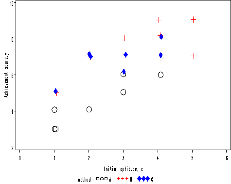
Table 6.13 on page 108.
proc glm data = table6_12;
  class method;
  model y = method x /intercept ss3;
run;
quit;
Dependent Variable: y
                                      Sum of
Source                     DF        Squares    Mean Square   F Value   Pr > F
Model                       4    870.6979592    217.6744898    359.20   <.0001
Error                      17     10.3020408      0.6060024
Uncorrected Total          21    881.0000000

R-Square     Coeff Var      Root MSE        y Mean
0.838550      12.47915      0.778462      6.238095

Source                     DF    Type III SS    Mean Square   F Value   Pr > F
Intercept                   1    58.05399323    58.05399323     95.80   <.0001
method                      2    16.93200174     8.46600087     13.97   0.0003
x                           1    16.55510204    16.55510204     27.32   <.0001