It is common to fit a model where a variable (or variables) has an effect on the expected mean. You may also want to fit a model where a variable has an effect on the variance, that is a model with heteroskedastic errors. One example is a hierarchical model where the error variance is not constant over some categorical variable (e.g. gender). Another example is a longitudinal model where you might want to allow the errors to vary across time. This page describes how to fit such a model and demonstrates with an example.
Example 1: Heteroskedastic errors by group
It may be useful to note that a multi-level model (or a single level model) that allows different error terms between groups is similar to a multi-group structural equation model in which all parameters in the model are constrained to equality except for the error terms.
The dataset for this example, hsb, includes data on 7185 students in 160 classrooms. The variable mathach is a measure of each student’s math achievement, the variable female is a binary variable equal to one if the student is female and zero otherwise, and the variable id contains the classroom identifier.
Below we run a model that uses female to predict mathach. This model assumes equal error variances for males and females.
proc mixed data = hsb method = ml;
  class id;
  model mathach = female / solution;
  random intercept/ subject = id type = cs;
run;

 Covariance Parameter Estimates
Cov Parm     Subject    Estimate
Variance     id           7.7108
CS           id           0.3982
Residual                 38.8448

           Fit Statistics
-2 Log Likelihood             47053.3
AIC (smaller is better)       47063.3
AICC (smaller is better)      47063.3
BIC (smaller is better)       47078.7

  Null Model Likelihood Ratio Test
    DF    Chi-Square      Pr > ChiSq
     2        936.66          <.0001

                   Solution for Fixed Effects
                         Standard
Effect       Estimate       Error      DF    t Value    Pr > |t|
Intercept     13.3453      0.2539     159      52.55      <.0001
female        -1.3594      0.1714    7024      -7.93      <.0001

        Type 3 Tests of Fixed Effects
              Num     Den
Effect         DF      DF    F Value    Pr > F
female          1    7024      62.89    <.0001
In order to fit a model with heteroskedastic errors, we must modify the above model. The model shown above can be written as:
mathach_ij = b0 + b1*female_ij + u_i + e_ij (1)
This model assumes:
e_ij ~ N(0,s2)
u_i ~ N(0,t2)
Where e_ij is the level 1 errors (i.e. residuals), and u_i is the random intercept across classrooms (i.e. the level 2 variance). We want to allow the variance of e_ij (i.e. s2) to be different for male and female students. One way to think about this would be to replace the single e_ij term, with separate terms for males and females, in equation form:
e_ij = e(m)_ij*male + e(f)_ij*female (2)
Where male is a dummy variable equal to one if the student is male and equal to zero otherwise, and e(m)_ij is the error term for males. The variable female and the term e(f)_ij are the same except that they are for females. Another way to write this is:
e_ij ~  N(0,s2_1)  females
        N(0,s2_2)  males
Another way to think about this is to use one group as the reference group, and estimate the difference between the variance of the two groups. In equation form this would be:
e_ij = e(f)_ij + e(m)_ij*male (3)
Where e(f)_ij is the error term for males, and e(m)_ij is the difference between the errors for males and females. This can also be written:
e_ij ~ N(0,s2 + s2_2*male)
This second way of looking at the error structure is part of how we will restructure our model to allow for heteroskedastic error terms.
Equation 3 says that the residual variance is a function of gender. So we can write it as r_ijk, where i is the group, j is the subject, and k is the gender.
mathach_ij = b0 + b1*female + u_i + r_ijk (4)
We can estimate the residual variance as a function of gender by using the repeated statement instead of random and using the local option in the repeated statement. This option adds a diagonal matrix to the variance-covariance matrix estimated in the model. We wish to estimate a variance parameter for gender. We will specify this effect as an exponential local effects and then go through the necessary transformations later to extract the estimated variance for each level of gender.
proc mixed data=hsb order = data method=ml;
  class female id;
  model mathach=female / solution ;
  repeated female /subject = id type = cs r local=exp(male);
run;

 Covariance Parameter Estimates
Cov Parm      Subject    Estimate
Variance      id           0.2929
CS            id           7.8810
EXP male                  0.09229
Residual                  37.0531

           Fit Statistics
-2 Log Likelihood             47044.4
AIC (smaller is better)       47056.4
AICC (smaller is better)      47056.4
BIC (smaller is better)       47074.9


  Null Model Likelihood Ratio Test
    DF    Chi-Square      Pr > ChiSq
     3        945.56          <.0001

                           Solution for Fixed Effects
                                         Standard
Effect       female          Estimate       Error      DF    t Value    Pr > |t|
Intercept                     13.3471      0.2568     159      51.96      <.0001
female                  1     -1.3759      0.1850     122      -7.44      <.0001
female                  0           0           .       .        .         .

        Type 3 Tests of Fixed Effects
              Num     Den
Effect         DF      DF    F Value    Pr > F
female          1     122      55.32    <.0001
The first table in the output shows the covariance parameter estimates. The residual variance for females is equal to Residual = 37.0531, while the variance for males is Residual*exp^(EXP male) = 37.0531*exp(0.09229) = 40.635498.
Example 2: A growth curve model
When you run a growth curve model in the structural equation modeling framework, it is not uncommon to allow the error variance to be different across time points, or at least to test whether such differences exist. A longitudinal model that allows different error variances across time points is similar to a growth model in the structural equation modeling setting, where all parameters except for the error terms across time points are constrained to equality. Below we show how to allow for different error variances across time points.
The example dataset contains data on 239 subjects. The dataset includes observations at up to five time points per subject, for a total of 1079 observations. The variable id uniquely identifies subjects. The time at which an observation was taken is indicated by the variable time, which takes on the values 0 to 4.
The example dataset, nys1, contains 1079 observations taken at up to five time points, nested within 239 subject. Although the example we use here is a longitudinal model, the same technique could be used for other types of clustered data, for example, students nested in classrooms. Below we use proc mixed to fit a model where the variables x, and time predict the variable attit. The variable time takes on five values, 0-4. The vi option in the random statement requests that variances of the random effects be reported in the output. The we specify method = ml indicating that the maximum likelihood estimator be used. We specify type = cs, indicating that we are fitting a model with compound symmetry in which the same variance-covariance is assumed for all times.
proc mixed data = nys1 method=ml;
  class id;
  model attit = x time /solution outpred = nys2;
  random intercept / subject=id type = cs vi;
run;

The Mixed Procedure

                  Model Information
Data Set                     WORK.NYS1
Dependent Variable           attit
Covariance Structure         Compound Symmetry
Subject Effect               id
Estimation Method            ML
Residual Variance Method     Profile
Fixed Effects SE Method      Model-Based
Degrees of Freedom Method    Containment

< ... output omitted ... >


 Covariance Parameter Estimates

Cov Parm     Subject    Estimate

Variance     id          0.02896
CS           id         0.001890
Residual                 0.03111


           Fit Statistics

-2 Log Likelihood              -280.6
AIC (smaller is better)        -268.6
AICC (smaller is better)       -268.5
BIC (smaller is better)        -247.8

  Null Model Likelihood Ratio Test
    DF    Chi-Square      Pr > ChiSq
     2        324.66          <.0001

                   Solution for Fixed Effects

                         Standard
Effect       Estimate       Error      DF    t Value    Pr > |t|
Intercept      0.1192     0.01849     238       6.45      <.0001
x             0.02412    0.003311     838       7.29      <.0001
time          0.06009    0.003956     838      15.19      <.0001

        Type 3 Tests of Fixed Effects
              Num     Den
Effect         DF      DF    F Value    Pr > F
x               1     838      53.10    <.0001
time            1     838     230.74    <.0001
The above model assumes that the residual errors are the same across time points, which may not be a reasonable assumption. In some cases, we may suspect heteroskedastic errors. In other cases, we may find them during our analysis. We can look at a boxplot of residuals at each time point to help us evaluate whether this is a reasonable assumption. From the proc mixed above, we have the residuals in the output dataset nys2. Below is the code to generate the boxplot.
proc sort data = nys2;
  by time;
run;
proc boxplot data = nys2;
  plot Resid * time;
run;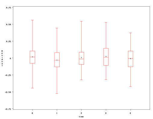
The graphs above show some differences in the residuals across time points, suggesting that we may want to model these differences. It is easier to understand what is going on if we look at the equations for our model. Our original model can be written as:
attit_ij = b0 + b1*x_ij + b2*time_ij + u_i + e_ij
Where u_i is the variance in the intercept across individuals (i.e. the level 2 variance), e_ij is the level 1 error variance. We want to allow e_ij to be different at each time point, in other words, we want to replace the single e_ij, with separate terms for each time point, in equation form:
e_ij = e(t0)_ij*time0 + e(t1)_ij*time1 + e(t2)_ij*time2 + e(t3)_ij*time3 + e(t4)_ij*time4
Where time0 is a dummy variable equal to one if time = 0 (i.e. the first time point) and equal to zero otherwise, and e(t0)_ij is the error for time 1. In other words, var(e_ij|time=0) = var(e(t0)_ij). The variables time1 to time4, are dummy variables for time equal one through four. The terms e(t1)_ij to e(t4)_ij are the error terms for time points 1-4.
Using some of the options in proc mixed, this model is doable in SAS, though the logic and interpretation require some careful thought. In order to model the heteroskedastic errors, we will be estimating the entries of a diagonal matrix to be added to the compound symmetry variance-covariance matrix. Each entry will correspond to a different time point. The "new" model can be written as:
attit_ijk = b0 + b1*x_ij + b2*time_ij + (b3 + e3_ij)*t1 + (b4 + e4_ij)*t2 + (b5 + e5_ij)*t3 + (b6 + e6_ij)*t4 + r_ijk
In the model above, t1 to t4 are dummy variables for the values of time, for example, when t1 = 1, when time=1, and zero otherwise. You may find it odd that the model includes both continuous time and a series of dummy variables representing time. The effect of the variable time is fixed, and it's coefficient, b2, is freely estimated. The model we will fit using proc mixed will use repeated instead of random. We can replicate the model we ran above by creating a categorical variable for time to be used in the repeated statement.
data nys1; set nys1;
  timecat = time;
run;

proc mixed data = nys1 method=ml;
  class id timecat;
  model attit = x time /solution;
  repeated timecat / subject=id type=cs;
run;

The Mixed Procedure

< ... output omitted ... >

 Covariance Parameter Estimates

Cov Parm     Subject    Estimate
CS           id          0.03085
Residual                 0.03111

           Fit Statistics
-2 Log Likelihood              -280.6
AIC (smaller is better)        -270.6
AICC (smaller is better)       -270.6
BIC (smaller is better)        -253.2


  Null Model Likelihood Ratio Test
    DF    Chi-Square      Pr > ChiSq
     1        324.66          <.0001

                   Solution for Fixed Effects
                         Standard
Effect       Estimate       Error      DF    t Value    Pr > |t|
Intercept      0.1192     0.01849     238       6.45      <.0001
x             0.02412    0.003311     838       7.29      <.0001
time          0.06009    0.003956     838      15.19      <.0001
To this model, we will add exercise the local option in the repeated statement. This option adds a diagonal matrix to the variance-covariance matrix estimated in the model. We wish to estimate a variance parameter for each time point. To do this, we will first create indicators for four of the five levels of our time variable. We will then enter these into the local statement. We will specify these as exponential local effects and then go through the necessary transformations later to extract the estimated variance for each level of time.
data nys1; set nys1;
  if time = 1 then ind2 = 1; else ind2 = 0;
  if time = 2 then ind3 = 1; else ind3 = 0;
  if time = 3 then ind4 = 1; else ind4 = 0;
  if time = 4 then ind5 = 1; else ind5 = 0;
run;

ods output  CovParms =t;
proc mixed data = nys1 method=ml;
  class id timecat;
  model attit = x time /solution;
  repeated timecat /subject=id type=cs r local=exp(ind2 ind3 ind4 ind5);
run;

The Mixed Procedure

< ... output omitted ... >

                 Estimated R Matrix for id 1006
 Row        Col1        Col2        Col3        Col4        Col5
   1     0.05286     0.02810     0.02810     0.02810     0.02810
   2     0.02810     0.05564     0.02810     0.02810     0.02810
   3     0.02810     0.02810     0.05870     0.02810     0.02810
   4     0.02810     0.02810     0.02810     0.06544     0.02810
   5     0.02810     0.02810     0.02810     0.02810     0.06640

 Covariance Parameter Estimates
Cov Parm      Subject    Estimate
Variance      id                0
CS            id          0.02810
EXP ind2                   0.1064
EXP ind3                   0.2117
EXP ind4                   0.4109
EXP ind5                   0.4362
Residual                  0.02476

           Fit Statistics
-2 Log Likelihood              -287.4
AIC (smaller is better)        -269.4
AICC (smaller is better)       -269.2
BIC (smaller is better)        -238.1

  Null Model Likelihood Ratio Test
    DF    Chi-Square      Pr > ChiSq
     5        331.40          <.0001

                   Solution for Fixed Effects
                         Standard
Effect       Estimate       Error      DF    t Value    Pr > |t|
Intercept      0.1208     0.01780     238       6.78      <.0001
x             0.02380    0.003306     838       7.20      <.0001
time          0.05976    0.003964     838      15.08      <.0001

        Type 3 Tests of Fixed Effects
              Num     Den
Effect         DF      DF    F Value    Pr > F
x               1     838      51.84    <.0001
time            1     838     227.27    <.0001
We have saved our covariance parameter estimates in a dataset t. We can look at the values here. The CS (compound symmetry) value we see is the off-diagonal entry of the R matrix in the model. The Residual estimate corresponds to the baseline error variance at time = 0. The other values presented are the exponential local effects. In the SAS code below, we calculate the error variances for the five time points.
proc print data = t;
run;

Obs    CovParm     Subject    Estimate
 1     Variance      id              0
 2     CS            id        0.02810
 3     EXP ind2                 0.1064
 4     EXP ind3                 0.2117
 5     EXP ind4                 0.4109
 6     EXP ind5                 0.4362
 7     Residual                0.02476

* sigma^2*exp(xb);
proc transpose data = t (drop=subject) prefix = _ out=twide;
  id covparm;
run;
proc print data = twide;
run;
                                               _EXP_       _EXP_       _EXP_       _EXP_
Obs     _NAME_     _Variance         _CS        ind2        ind3        ind4        ind5    _Residual
 1     Estimate           0      0.02810      0.1064      0.2117      0.4109      0.4362     0.02476

data twidea;
  set twide;
  array sigma(5);
  array b(4) _exp_ind2 - _exp_ind5;
  do i = 2 to 5;
    sigma(i) = _residual*exp(b[i-1]);
  end;
  sigma1 = _residual;
run;
proc print data = twidea;
 var sigma:;
run;

Obs     sigma1      sigma2      sigma3      sigma4      sigma5
 1     0.024761    0.027541    0.030600    0.037345    0.038301