Introduction to R
IDRE Statistical Consulting Group
Background
Purpose of this seminar
This seminar introduces the funtionality of R, with a focus on data analysis.
In this seminar we will learn:
- how to interact with
R through RStudio
- a bit of
R coding
- tools to import, clean, manage, and export data
- simple data analysis functions
- the basics of two
R graphical systems
- how to use
R to share your data analysis with others
Coding instructions to help you learn R will appear in boxes like this.
R as a programming environment
R is a programming environment for statistical computing and graphics.
R
- serves as a data analysis and storage facility
- is designed to perform operations on vectors and matrices
- uses a well-developed but simple programming language (called
S)
- allows for rapid development of new tools according to user demand
These tools are distributed as packages, which any user can download to customize the R environment.
Why (and why not) R?
R has many advantages as data analysis software:
- Free
- Free online books to learn R
- online community is much larger than those for other statistical software
- Powerful, intuitive graphics systems make it easy to produce publication-quality graphics
- Easily create data analysis reports as documents and presentations for reproducibility with R Markdown
- Many specialized packages featuring analysis tools not available in other software
R also has a few disadvantages:
- somewhat more difficult to master than other statistical software
- frequent updates require maintenance
RStudio
RStudio
You can work directly in R, but most users prefer a graphical interface. We highly recommend using RStudio, an integrated development environment (IDE) that features:
- a console
- a powerful code/script editor featuring
- special tools for plotting, viewing R objects and code history
- cheatsheets for R programming
- tab-completion for object names and function arguments (enough reason by itself!)
RStudio Console
You can input and execute commands directly in the console.
Output of commands will typically be displayed in the console.
The RStudio console features tab-code-completion and live help for function coding.
Type rno into the RStudio console, wait a second, and when a window with rnorm appears, hit the Tab key.
Once you have the rnorm() function name completed, if the cursor is inside of (), RStudio will remind you of the the function’s arguments in a window . You can also hit the Tab key to see and issue the function argument names.
Place the cursor inside of rnorm(). Hit the Tab key twice, and then type the number 10. Hit Enter to execute the code.
You have just randomly generated 10 normally-distributed numbers.
RStudio Script Editor
Most R programs written for data analysis consists of many commands, making entering code line-by-line into the console inefficient.
Instead, we use the script editor to save our commands as a record of the steps we took to analyze our data. We can also issue R commands directly from the editor.
The script editor features the same tab-code-completion and function help as the console, as well as syntax highlighting.
If you do not see the script editor already open, open it now by selecting File > New File > R Script.
Write the code 1 + 2 in the script editor.
On the next line, type the code log. When the tab-completion window appears with a list of possible commands, hit Tab to choose log(). Enter 10 inside the ().
To execute code directly from the script editor, place the cursor inside the command (or highlight the entire command), and then hit Ctrl-Enter (on PCs, use Command-Enter on Macs). This will advance the cursor to the next command, where you can hit Ctrl-Enter again to run it, advancing the cursor to the next command…
Execute the two commands in the script editor using the keyboard shortcuts.
Make sure to periodically save your scripts. Most R scripts are saved with the .R extension.
Save your R script with the name mycode.R.
Unless otherwise specified, all coding instructions for this seminar should be entered into the script editor.
RStudio Environment pane
R stores both data and output from data analysis (as well as everything else) in objects.
Data are assigned to and stored in objects using the <- or = operator.
In the script editor, issue the code x <- 5 to create our first object.
Once you create an object, it should appear in the RStudio Environment pane.
To print the contents of an object to the console, specify the object’s name alone.
Specify and execute the code x to view the contents of x in the console.
Help for R and RStudio
The RStudio Help menu contains links to many documents for help with both R (select R Help) and RStudio (see RStudio Docs and RStduio Community Forum).
We particularly like the Cheatsheets, which are compact documents crammed with useful information on how to use various products made by the RStudio group.
Open the cheatsheet for RStudio by selecting the Help menu -> Cheatsheets -> RStudio IDE Cheat Sheet. Note the cheatsheet will usually be downloaded in a web browser as a .pdf.
Working with R packages
Base R and packages
Base R and most R packages are available for download from the Comprehensive R Archive Network (CRAN)
- cran.r-project.org
- base
R comes with a number of basic data management, analysis, and graphical tools
- However,
R’s power and flexibility lie in its array of packages (currently more than 15,000 on CRAN!)
Installing packages
To use packages in R, we must first install them using the install.packages() function, which typically downloads the package from CRAN and installs it for use.
Use the argument dependencies=TRUE to load all other packages required by the targeted package.
# uncomment (remove ##) to run
install.packages("dplyr", dependencies=TRUE)
install.packages("ggplot2", dependencies=TRUE)
install.packages("rmarkdown", dependencies=TRUE)
install.packages("shiny", dependencies=TRUE)
If you have not installed them already, please install dplyr, ggplot2, rmarkdown, and shiny with the necessary dependencies.
Loading packages
After installing a package, we can load it into the R environment using the library() or require() functions, which more or less do the same thing.
Functions and data structures within the package will then be available for use.
library(dplyr)
library(ggplot2)
library(shiny)
Load the package dplyr into your session now with library().
Vignettes *
Many packages include vignettes – longer, tutorial style guides for a package.
To see a list of available vignettes for the packages that are loaded, use vignette() with no arguments. Then to view a vignette, place its name inside vignette():
# list all available vignettes
vignette()
View the “Introduction to dplyr” vignette by issuing the command vignette("dplyr").
Basic R coding
R programming 1: Coding
Remember that we assign data to objects with <- or =.
Character data (i.e. strings) are surrounded by " or '.
In the script editor, create an object named a and assign it the character string “hello”.
Commands are separated either by a ; or by a newline.
R is case sensitive.
The # character at the beginning of a line signifies a comment, which is not executed.
On the next line, create an object named b, assign it the logarithm of 10 (using the log() function), but put a # at the beginning of the line. What happens when you try to execute this line?
Commands can extend beyond one line of text. Put operators like + at the end of lines for multi-line commands.
# Put operators like + at the end of lines
2 +
  3
## [1] 5
R programming 2: Functions and help files
Functions perform most of the work on data in R.
Functions in R are much the same as they are in math – they perform some operation on an input and return some output. For example, the mathematical function \(f(x) = x^2\), takes an input \(x\), and returns its square. Similarly, the mean() function in R takes a vector of numbers and returns its mean.
The inputs to functions are often referred to as arguments.
Help files for R functions are accessed by preceding the name of the function with ?.
Try opening the help file for log() with the code ?log.
In the help file, we will find the following useful sections:
- Description: overview of the function
- Usage: syntax, with list of arguments in particular order
- Arguments: description of arguments
- Details: in depth description of function’s operation
- Value: output of the function
- Examples: copy-and-pasteable examples
R programming 3: Function arguments
Values for arguments to functions can be specified either by name or position.
For log(), we see the first argument is x, the number whose log we want to take, and the second is base, the base of the logarithm.
# specifying arguments by name
log(x=100, base=10)
## [1] 2

# specifying arguments by position
log(8, 2)
## [1] 3
In the help file Usage section, if something is specified after an argument’s name and =, it is the default value.
In the log() help file, we see that the default value for base is exp(1), or \(e\), making log() a natural logarithm function by default.
Vectors
Vectors, the fundamental data structure in R, are one-dimensional and homogeneous.
A single variable can usually be represented by one of the following vector data types:
- logical: TRUE or FALSE (1 or 0)
- integer: integers only (represented by a number followed by L; e.g. 10L is the integer 10)
- double: real numbers, also known as numeric
- character: strings
A single value is a vector of length one in R.
Creating vectors
The c() function combines values of common type together to form a vector.
# create a vector
first_vec <- c(1, 3, 5)
first_vec
## [1] 1 3 5

# length() returns the number of elements
char_vec <- c("these", "are", "some", "words")
length(char_vec)
## [1] 4

# the result of this comparison is a logical vector
first_vec > c(2, 2, 2)
## [1] FALSE  TRUE  TRUE
To create vectors with a predictable sequence of elements, use rep() for repeating elements and seq() for sequential elements.
The expression m:n will generate a vector of integers from m to n
# first argument to rep is what to repeate
# the second argument is number of repetitions
rep(0, times=3)
## [1] 0 0 0
rep("abc", 4)
## [1] "abc" "abc" "abc" "abc"

# arguments for seq are from, to, by
seq(from=1, to=5, by=2)
## [1] 1 3 5
seq(10, 0, -5)
## [1] 10  5  0

# colon operator
3:7
## [1] 3 4 5 6 7

# you can nest functions
rep(seq(1,3,1), times=2)
## [1] 1 2 3 1 2 3
Create the vector (4,5,6) in three different ways using c(), seq(), and the : operator.
Try creating the vector (2,2,1,1) in at least two different ways.
Subsetting vectors with []
Elements of a vector can be accessed or subset by specifying a vector of numbers (of length 1 or greater) inside [].
# create a vector 10 to 1
# putting () around a command will cause the result to be printed
(a <- seq(10,1,-1))
##  [1] 10  9  8  7  6  5  4  3  2  1

# second element
a[2]
## [1] 9

# first 5 elements
a[seq(1,5)]
## [1] 10  9  8  7  6

# first, third, and fourth elements
a[c(1,3,4)]
## [1] 10  8  7
Create the vector y as the integers counting down from 10 to 1. Extract the second, fifth, and seventh element of this vector y.
Conditional selection - subsetting by value
Vectors elements can also be subset with a logical (TRUE/FALSE) vector, known as logical subsetting.
scores <- c(55, 24, 43, 10)
scores[c(FALSE, TRUE, TRUE, FALSE)]
## [1] 24 43
This allows us to subset a vector by checking if a condition is satisifed:
# this returns a logical vector...
scores < 30
## [1] FALSE  TRUE FALSE  TRUE

# ...that we can now use to subset
scores[scores<30]
## [1] 24 10
Use conditional selection to find the numbers in y (integers from 10 to 1) that when multiplied by 2, the result is greater than 15.
Importing and Exporting Data
Dataset files
R works most easily with datasets stored as text files. Typically, values in text files are separated, or delimited, by tabs or spaces:
gender id race ses schtyp prgtype read write math science socst
0 70 4 1 1 general 57 52 41 47 57
1 121 4 2 1 vocati 68 59 53 63 31
0 86 4 3 1 general 44 33 54 58 31
0 141 4 3 1 vocati 63 44 47 53 56
or by commas (CSV file):
gender,id,race,ses,schtyp,prgtype,read,write,math,science,socst
0,70,4,1,1,general,57,52,41,47,57
1,121,4,2,1,vocati,68,59,53,63,61
0,86,4,3,1,general,44,33,54,58,31
0,141,4,3,1,vocati,63,44,47,53,56
Reading in text data
R provides several related functions to read data stored as files.
Use read.csv() to read in data stored as CSV and read.delim() to read in text data delimited by other characters (such as tabs or spaces).
For read.delim(), specify the delimiter in the sep= argument.
Both read.csv() and read.delim() assume the first row of the text file is a row of variable names. If this is not true, use the argument header=FALSE.
Although we are retrieving files over the internet for this class, these functions are typically used for files saved to disk.
Note how we are assigning the loaded data to objects.
# basic syntax of read.csv, not run
data <- read.csv("/path/to/file.csv")

# specification for tab-delimited file
dat.tab <- read.delim("/path/to/file.txt",  sep="\t")
Create a dataset called dat_csv by loading a dataset from our server at this address: https://stats.idre.ucla.edu/stat/data/hsbraw.csv .
dat_csv <- read.csv("https://stats.idre.ucla.edu/stat/data/hsbraw.csv")
Exporting data
We can export our data to a .csv file with write.csv().
If you need to save multiple objects from your session, you can save whatever objects you need with save(), which creates a binary .Rdata file, which can loaded for later use with load().
We did not specify realistic pathnames below.
# write a csv file
write.csv(dat_csv, file = "path/to/save/filename.csv")

# save these objects to an .Rdata file
save(dat_csv, mydata, file="path/to/save/filename.Rdata")
Packages for importing
Packages to read and write data in other software formats:
readxl : Excel fileshaven: Stata, SAS, and SPSS
The readr package contains updated versions of read.csv() and read.delim() (called read_csv() and read_delim()) that use modernized data structures
Data Frames
Data frames
Data sets for statistical analysis are typically stored in data frames in R. The objects created by read.csv() and read.table() are data frames.
Data frames are rectangular, where the columns are variables and the rows are observations of those variables.
Data frame columns can be of different data types (some double, some character, etc.) – but they must be equal length
Real datasets usually combine variables of different types, so data frames are well suited for storage.
Viewing data as a spreadsheet with View(), head() and tail()
Use View() on a dataset to open a spreadsheet-style view of a dataset. In RStuido, clicking on a dataset in the Environment pane will View() it.
View the dataset dat_csv.
For large data files, use head() and tail() to look at a specified number of rows at the begininning or end of a dataset, respectively.
# first 2 rows
head(dat_csv, 2)
##    id female    ses schtyp     prog read write math science socst       honors
## 1  45 female    low public vocation   34    35   41      29    26 not enrolled
## 2 108   male middle public  general   34    33   41      36    36 not enrolled
##   awards cid
## 1      0   1
## 2      0   1
# last 8 rows
tail(dat_csv, 8)
##      id female    ses  schtyp     prog read write math science socst
## 193 174   male middle private academic   68    59   71      66    56
## 194  95   male   high  public academic   73    60   71      61    71
## 195  61 female   high  public academic   76    63   60     -99   -99
## 196 100 female   high  public academic   63    65   71      69    71
## 197 143   male middle  public vocation   63    63   75      72    66
## 198  68   male middle  public academic   73    67   71      63    66
## 199  57 female middle  public academic   71    65   72      66    56
## 200 132   male middle  public academic   73    62   73      69    66
##           honors awards cid
## 193 not enrolled      2  20
## 194     enrolled      2  20
## 195     enrolled      4  20
## 196                 -99  20
## 197     enrolled      4  20
## 198     enrolled      7  20
## 199     enrolled      5  20
## 200     enrolled      3  20
Subsetting data frames
With a two-dimensional structure, data frames can be subset with matrix notation [rows, columns].
Use vectors to subset multiple rows/columns.
Omitting rows or columns specifies all rows and columns, respectively.
# use data.frame() to create a data frame manually
mydata <- data.frame(patient=c("Smith", "Jones", "Williams"),
                     height=c(72, 61, 66),
                     diabetic=c(TRUE, FALSE, FALSE))


# row 3 column 2
mydata[3,2]
## [1] 66

# first two rows of column height
mydata[1:2, "height"]
## [1] 72 61

# all rows of column diabetic
mydata[,"diabetic"]
## [1]  TRUE FALSE FALSE
Extract the 2nd, 5th, and 10th rows of the variable math in the dat_csv data set.
Variables, or columns, of a data frame can be selected with the $ operator, and the resulting object is a vector.
We can further subset elements of the selected column vector using [].
# subsetting creates a numeric vector
mydata$height
## [1] 72 61 66

# just the second and third elements
mydata$height[2:3]
## [1] 61 66
Extract the 2nd, 5th, and 10th rows of the variable math in the dat_csv data set using the $ operator
Naming data frame columns
colnames(data_frame) returns the column names of data_frame (or matrix).
colnames(data_frame) <- c("some", "names") assigns column names to data_frame.
# get column names
colnames(mydata)
## [1] "patient"  "height"   "diabetic"

# assign column names (capitalizing them)
colnames(mydata) <- c("Patient", "Height", "Diabetic")
colnames(mydata)
## [1] "Patient"  "Height"   "Diabetic"

# to change one variable name, just use vector indexing
colnames(mydata)[3] <- "Diabetes"
colnames(mydata)
## [1] "Patient"  "Height"   "Diabetes"
Examining the structure of an object
Use dim() on two-dimensional objects to get the number of rows and columns.
Use str(), to see the structure of the object, including its class and the data types of elements. We also see the first few rows of each variable.
# number of rows and columns
dim(mydata)
## [1] 3 3

#d is of class "data.frame"
#all of its variables are of type "integer"
str(mydata)
## 'data.frame':    3 obs. of  3 variables:
##  $ Patient : chr  "Smith" "Jones" "Williams"
##  $ Height  : num  72 61 66
##  $ Diabetes: logi  TRUE FALSE FALSE
Examine the structure of dat_csv with str().
Adding new variables to the data frame
You can add variables to data frames by declaring them to be column variables of the data frame as they are created.
Trying to add a column of the wrong length will result in an error.
# this will add a column variable called logwrite to d
mydata$logHeight <- log(mydata$Height)

# now we see logwrite as a column in d
colnames(mydata)
## [1] "Patient"   "Height"    "Diabetes"  "logHeight"

# d has 200 rows, and the rep vector has 300
mydata$z <- rep(0, 5)
## Error in `$<-.data.frame`(`*tmp*`, z, value = c(0, 0, 0, 0, 0)): replacement has 5 rows, data has 3
Here are some useful functions to create variables from existing variables:
log(): logarithmmin_rank(): rank valuescut(): cut a continuous variable into intervals with new integer value signifying into which interval original value falls
scale(): standardizes variable (substracts mean and divides by standard deviation)lag(), lead(): lag and lead a variablecumsum(): cumulative sumrowMeans(), rowSums(): means and sums of several columns
Create a data set called test3 that is all rows of the 3 column variables math, read, and write from dat_csv.
Add a variable to test3 called test_mean that is the mean of the variables math, read, and write. Specify the data.frame test3 as the only argument to rowMeans().
Use head() to look at the first 5 rows of test3.
Data Management
Preparing data for analysis
Taking the time to prepare your data before analysis can save you frustration and time spent cleaning up errors:
- Cut the data set down to only those observations (rows) and variables (columns) needed for analysis
- Combining data sets
- Make sure variable values are free of errors, such as impossible values or numeric codes for missing values
The package dplyr contains several easy-to-use data management functions that we will learn to use to manage our data.
# load packages for this section
library(dplyr)
If you have not already, load dplyr into the current session with library().
Subsetting rows of a data frame with filter()
The dplyr function filter() will subset the rows (observations) of a data frame according to some condition (e.g. all rows where a column value is greater than x, all rows where a column value is equal to y).
# creating some data manually
dog_data <- data.frame(id = c("Duke", "Lucy", "Buddy", "Daisy", "Bear", "Stella"),
                       weight = c(25, 12, 58, 67, 33, 9),
                       sex=c("M", "F", "M", "F", "M", "F"),
                       location=c("north", "west", "north", "south", "west", "west"))


# dogs weighing more than 40
filter(dog_data, weight > 40)
##      id weight sex location
## 1 Buddy     58   M    north
## 2 Daisy     67   F    south

# female dogs in the north or south locations
filter(dog_data, (location == "north" | location == "south") & sex == "F")
##      id weight sex location
## 1 Daisy     67   F    south
Create a data set from dat_csv called low_read that contains observations where the read score is less than or equal to 50.
Create a data set from dat_csv called mid_read that contains observations where the read score is greater than 50 but also less than or equal to 60.
Subsetting Variables (columns)
Often, datasets come with many more variable than we want. We can use the dplyr function select() to keep only the variables we need.
# select 2 variables
select(dog_data, id, sex)
##       id sex
## 1   Duke   M
## 2   Lucy   F
## 3  Buddy   M
## 4  Daisy   F
## 5   Bear   M
## 6 Stella   F
Use - to unselect (select out) columns.
# select everything BUT id and sex
select(dog_data, -c(id, sex))
##   weight location
## 1     25    north
## 2     12     west
## 3     58    north
## 4     67    south
## 5     33     west
## 6      9     west
Create a data set called high_read_in that is just the id and read variables for observations where read is greater than 60. Create another data set called high_read_out that is all of the other variables besides read (include id in both data sets) for the same observations with read greater than 60.
Appending observations (appending by rows)
Sometimes we are given our dataset in parts, with observations spread over many files (collected by different researchers, for example). To create one dataset, we need to append the datasets together row-wise.
The function rbind() appends data frames together. The variables must be the same between datasets.
Here, we rbind() a new data set of dogs, more_dogs, to our current dog_data.
# make a data.frame of new dogs
more_dogs <- data.frame(id = c("Jack", "Luna"),
                        weight=c(38, -99),
                        sex=c("M", "F"),
                        location=c("east", "east"))


# make sure that data frames have the same columns
names(dog_data)
## [1] "id"       "weight"   "sex"      "location"
names(more_dogs)
## [1] "id"       "weight"   "sex"      "location"

# appended dataset combines rows
all_dogs <- rbind(dog_data, more_dogs)
all_dogs
##       id weight sex location
## 1   Duke     25   M    north
## 2   Lucy     12   F     west
## 3  Buddy     58   M    north
## 4  Daisy     67   F    south
## 5   Bear     33   M     west
## 6 Stella      9   F     west
## 7   Jack     38   M     east
## 8   Luna    -99   F     east
Append low_read and mid_read and call the resulting data set low_and_mid_read. Check in the Environment pane that low_and_mid_read has the correct number of observations.
Adding data columns by merging on a key variable *
We often receive separate datasets with different variables (columns) that must be merged on a key variable.
Merging is an involved topic, with many different kinds of merges possible, depending on whether every observation in one dataset can be matched to an observation in the other dataset. Sometimes, you’ll want to keep observations in one dataset, even if it is not matched. Other times, you will not.
We will solely demonstrate merges where only matched observations are kept.
We will use the dplyr function inner_join() to perform the merge. The base R function merge() can be used for the same type of merge.
inner_join() will search both datasets for any variables with the same name, and will use those as matching variables. If you need to control which variables are used to match, use the by= argument.
# new dog variable
# matching variables do not have to be sorted
dog_vax <- data.frame(id = c("Luna", "Duke", "Buddy", "Stella", "Daisy", "Lucy", "Jack", "Bear"),
                      vaccinated = c(TRUE, TRUE, TRUE, TRUE, TRUE, FALSE, FALSE, FALSE))

# id appears in both datasets, so will be used to match observations
dogs <- inner_join(all_dogs, dog_vax)
## Joining, by = "id"
dogs
##       id weight sex location vaccinated
## 1   Duke     25   M    north       TRUE
## 2   Lucy     12   F     west      FALSE
## 3  Buddy     58   M    north       TRUE
## 4  Daisy     67   F    south       TRUE
## 5   Bear     33   M     west      FALSE
## 6 Stella      9   F     west       TRUE
## 7   Jack     38   M     east      FALSE
## 8   Luna    -99   F     east       TRUE
Merge high_read_in and high_read_out and call it high_read.
Append high_read to low_and_mid_read and call it all_read. Check in the Environment pane that all_read and dat_csv are the same size.
Missing values
Missing values in R are represented by the reserved symbol NA (cannot be used for variable names).
Blank fields in a text file will generally be converted to NA when loaded into R.
Often, datasets use codes, such as impossible numeric values (e.g. -99) to denote missing values.
We can convert missing data codes like -99 in variables to NA with conditional selection.
# subset to science values equal to -99, and then change
#  them all to NA
dogs$weight[dogs$weight == -99] <- NA
dogs$weight
## [1] 25 12 58 67 33  9 38 NA
Missing values are contagious
In R, NA means “undefined”, so most operations involving an NA value will result in NA (as the result is “undefined”):
# a sum involving "undefined" is "undefined"
1 + 2 + NA
## [1] NA

# NA could be larger or smaller or equal to 2
c(1, 2, 3, NA) > 2
## [1] FALSE FALSE  TRUE    NA

# mean is undefined because of the presence of NA
dogs$weight
## [1] 25 12 58 67 33  9 38 NA
mean(dogs$weight)
## [1] NA
However, many functions allow the argument na.rm (or soemthing similar) to be set to TRUE, which will first remove any NA values from the operation before calculating the result:
# NA values will be removed first
sum(c(1,2,NA), na.rm=TRUE)
## [1] 3

mean(dogs$weight, na.rm=TRUE)
## [1] 34.57143
You cannot check for equality to NA because means “undefined”. It will always result in NA.
Use is.na() instead.
# one of the values is NA
x <- c(1, 2, NA)

# check for equality to NA using == is wrong
# RStudio may give you a warning about this (to use is.na() instead)
x == NA
## [1] NA NA NA

# this is correct
is.na(x)
## [1] FALSE FALSE  TRUE
In dat_csv, the variable science contains -99 values to signify missing. How can you identify which rows have -99 values?
Convert all of these -99 values to NA.
Calculate the mean of science ignoring the missing values.
Basic Data Analysis
Descriptive statistics for continuous variables
Common numeric summaries for continuous variables are the mean, median, and variance, obtained with mean(), median(), and var() (sd() for standard deviation), respectively.
summary() on a numeric vector provides the min, max, mean, median, and first and third quartiles (interquartile range).
# create a new bloodtest data set
bloodtest <- data.frame(id = 1:10,
                        gender = c("female", "male", "female", "female", "female", "male", "male", "female", "male", "female"),
                        hospital = c("CLH", "MH", "MH", "MH", "CLH", "MH", "MDH", "MDH", "CLH", "MH"),
                        doc_id = c(1, 1, 1, 2, 2, 2, 3, 3, 3, 3),
                        insured = c(0, 1, 1, 1, 0, 1, 1, 0, 1, 1),
                        age = c(23, 45, 37, 49, 51, 55, 56, 37, 26, 40),
                        test1  = c(47, 67, 41, 65, 60, 52, 68, 37, 44, 44),
                        test2 = c(46, 57, 47, 65, 62, 51 ,62 ,44 ,46, 61),
                        test3 = c(49, 73, 50, 64, 77, 57, 75, 55, 62, 55),
                        test4 = c(61, 61, 51, 71, 56, 57, 61, 46, 46, 46))


mean(bloodtest$age)
## [1] 41.9
median(bloodtest$age)
## [1] 42.5
var(bloodtest$age)
## [1] 130.5444

summary(bloodtest$test1)
##    Min. 1st Qu.  Median    Mean 3rd Qu.    Max.
##   37.00   44.00   49.50   52.50   63.75   68.00
Correlations
Correlations provide quick assessments of whether two continuous variables are linearly related to one another.
The cor() function estimates correlations. If supplied with 2 vectors, cor() will estimate a single correlation. If supplied a data frame with several variables, cor() will estimate a correlation matrix.
# just a single correlation
cor(bloodtest$test1, bloodtest$test2)
## [1] 0.7725677

# use dplyr select() to pull out just the test variables
scores <- select(bloodtest, test1, test2, test3, test4)
cor(scores)
##           test1     test2     test3     test4
## test1 1.0000000 0.7725677 0.8174523 0.7959618
## test2 0.7725677 1.0000000 0.6691743 0.5298743
## test3 0.8174523 0.6691743 1.0000000 0.3612138
## test4 0.7959618 0.5298743 0.3612138 1.0000000
Create a correlation table of the dat_csv variables read, write, math, science, and socst.
Frequency tables
The statistics mean, median and variance cannot be calculated meaningfully for categorical variables (unless just 2 categories).
Instead, we often present frequency tables of the distribution of membership to each category.
Use table() to produce frequency tables.
Use prop.table() on the tables produced by table() (i.e. the output) to see the frequencies expressed as proportions.
Some of the categorical variables in this dataset are:
# table() produces counts
table(bloodtest$gender)
##
## female   male
##      6      4
table(bloodtest$hospital)
##
## CLH MDH  MH
##   3   2   5

# for proportions, use output of table()
#   as input to prop.table()
prop.table(table(bloodtest$hospital))
##
## CLH MDH  MH
## 0.3 0.2 0.5
Crosstabs
Two-way and multi-way frequency tables (crosstabs) are used to explore the relationships between categorical variables.
We can use table() and prop.table() again. Within prob.table(), use margin=1 for row proportions and margin=2 for column proportions. Omitting margin= will give proportions of the total.
# this time saving the freq table to an object
my2way <- table(bloodtest$gender, bloodtest$hospital)

# counts in each crossing of prog and ses
my2way
##
##          CLH MDH MH
##   female   2   1  3
##   male     1   1  2

# row proportions,
#   proportion of prog that falls into ses
prop.table(my2way, margin=1)
##
##                CLH       MDH        MH
##   female 0.3333333 0.1666667 0.5000000
##   male   0.2500000 0.2500000 0.5000000

# columns proportions,
#   proportion of ses that falls into prog
prop.table(my2way, margin=2)
##
##                CLH       MDH        MH
##   female 0.6666667 0.5000000 0.6000000
##   male   0.3333333 0.5000000 0.4000000
Determine the proportion of each socio-economic group (variable ses) within each school type (variable schtyp) in the dat_csv data set.
Statistical analysis in R
The stats package, loaded with base R, provides a wide array of commonly used statistical tools, including:
- chi-square tests and several related/similar tests
- t-tests
- correlation and covariance
- ANOVA and linear regression models
- generalized linear regression models (logistic, poisson, etc.)
- time series analysis
- statistical distributions (random numbers, density, distribution, and quantile functions)
Even more tools are available in various downloadable packages.
We will be covering only tools available in stats in this seminar.
Chi-square test of indepedence
Chi-square tests are often used to test for association between two categorical variables. It tests whether the proportions of membership to categories of one variable are related to the proportion of membership to categories of another variable.
Use chisq.test() to perform the chi-square test of independence. Supply two categorical variables (can be numeric or character) as arguments.
Here we test whether hospital and being insured are independent.
# program and ses class appear to be associated
chisq.test(bloodtest$hospital, bloodtest$insured)
## Warning in chisq.test(bloodtest$hospital, bloodtest$insured): Chi-squared
## approximation may be incorrect
##
##  Pearson's Chi-squared test
##
## data:  bloodtest$hospital and bloodtest$insured
## X-squared = 4.4444, df = 2, p-value = 0.1084
Because some of our expected cell sizes are less than 5, R warns us that the chi-squared test may not be close to exact.
Independent samples t tests
Two sample t-tests model a simple relationship – that the mean of an outcome variable (assumed to be normally distributed) is associated with a two-group predictor variable.
Use t.test() with formula notation to perform an independent samples t-test of whether test1 score is associated with gender:
# formula notation for independent samples t-test
t.test(test1 ~ gender, data=bloodtest)
##
##  Welch Two Sample t-test
##
## data:  test1 by gender
## t = -1.1813, df = 6.2951, p-value = 0.2802
## alternative hypothesis: true difference in means is not equal to 0
## 95 percent confidence interval:
##  -26.670132   9.170132
## sample estimates:
## mean in group female   mean in group male
##                49.00                57.75
Test1 score does not appear to differ between the genders.
Perform a t-test to determine whether math scores are different between genders (variable female) with data set dat_csv.
Paired samples t test
With a paired samples (dependent samples) t-test, we test whether the means of two possibly correlated variables are different.
Below we use t.test() to test whether the means of patients’ test1 and test3 scores tend to be different. For a paired test, do not use formula notation, but instead specify two vectors of equal length and paired=TRUE.
t.test(bloodtest$test1, bloodtest$test3, paired=TRUE)
##
##  Paired t-test
##
## data:  bloodtest$test1 and bloodtest$test3
## t = -4.3231, df = 9, p-value = 0.001925
## alternative hypothesis: true difference in means is not equal to 0
## 95 percent confidence interval:
##  -14.014139  -4.385861
## sample estimates:
## mean of the differences
##                    -9.2
The paired t-test suggests that test3 scores are significantly different from test1 scores.
Linear regression
Linear regression expands the simple predictor-outcome model of t-tests by allowing more predictors. These predictors be distribtued in any way (not just binary predictors).
The lm() function is used to fit linear regression models.
Numeric and character variable predictors are acceptable. Character variables are essentially treated as factors (categorical variables), where by default, a dummy (0/1) variable is entered into the model for each level except for the first.
Below we fit a model where we predict a patients’s test1 score from their age and gender, and store the model as an object.
# fit a linear model (ANOVA and linear regression)
m1 <- lm(test1 ~ age + gender, data=bloodtest)
# printing an lm object will list the coefficients only
m1
##
## Call:
## lm(formula = test1 ~ age + gender, data = bloodtest)
##
## Coefficients:
## (Intercept)          age   gendermale
##     24.4871       0.6206       5.0265
Model objects and extractor functions
Model objects, the output of regression model fitting functions like lm(), are usually too complex to examine directly, as they contain an abundance of diverse information related to the the fitted model.
Instead, we often use a set of extractor functions to pull out the desired information from a model object.
summary(): regression table of coefficients, standard errors, test statistics, and p-values, as well as overall model fit statisticscoef(): just model coefficientsresiduals(): residualspredict(): predictions based on fitted modelconfint(): confidence intervals for coefficients
These functions will often (but not always) work with model objects fit with functions other than lm().
# summary produces regression table and model fit stats
summary(m1)
##
## Call:
## lm(formula = test1 ~ age + gender, data = bloodtest)
##
## Residuals:
##     Min      1Q  Median      3Q     Max
## -11.646  -6.164   1.043   7.146  10.104
##
## Coefficients:
##             Estimate Std. Error t value Pr(>|t|)
## (Intercept)  24.4871    11.7845   2.078   0.0763 .
## age           0.6206     0.2824   2.198   0.0639 .
## gendermale    5.0265     6.2477   0.805   0.4475
## ---
## Signif. codes:  0 '***' 0.001 '**' 0.01 '*' 0.05 '.' 0.1 ' ' 1
##
## Residual standard error: 9.316 on 7 degrees of freedom
## Multiple R-squared:  0.4981, Adjusted R-squared:  0.3547
## F-statistic: 3.474 on 2 and 7 DF,  p-value: 0.08957
Peform a linear regression of the outcome read with predictors math, female, and ses using dat_csv. Call the model object m1. Interpret your results.
# just the coefficients
coef(m1)
## (Intercept)         age  gendermale
##  24.4871383   0.6205788   5.0265273

# 95% confidence intervals
confint(m1)
##                   2.5 %    97.5 %
## (Intercept) -3.37869862 52.352975
## age         -0.04713382  1.288291
## gendermale  -9.74700686 19.800062

# first 5 observed values, predicted values and residuals
# cbind() joins column vectors into a matrix
cbind(bloodtest$test1, predict(m1), residuals(m1))
##    [,1]     [,2]       [,3]
## 1    47 38.76045   8.239550
## 2    67 57.43971   9.560289
## 3    41 47.44855  -6.448553
## 4    65 54.89550  10.104502
## 5    60 56.13666   3.863344
## 6    52 63.64550 -11.645498
## 7    68 64.26608   3.733923
## 8    37 47.44855 -10.448553
## 9    44 45.64871  -1.648714
## 10   44 49.31029  -5.310289
ANOVA *
When an object of class lm is supplied to anova(), an analysis of variance table of the fitted model is produced. The ANOVA partioning uses sequential sums of squares (Type I SS), so if other sums of squares are desired, see the Anova() function in the car package.
# ANOVA sequential sums of squares
anova(m1)
## Analysis of Variance Table
##
## Response: test1
##           Df Sum Sq Mean Sq F value Pr(>F)
## age        1 546.77  546.77  6.2997 0.0404 *
## gender     1  56.18   56.18  0.6473 0.4475
## Residuals  7 607.55   86.79
## ---
## Signif. codes:  0 '***' 0.001 '**' 0.01 '*' 0.05 '.' 0.1 ' ' 1
The anova() function is often used to conduct a likelihood ratio test, that compares the fit of nested models to the data. This test allows one to assess whether the addition of several predictors improves the fit of the model.
Simply specify two nested models to anova() to conduct the likelihood ratio test:
# fit another linear regression model, adding hosiptal as predictor (two parameters added to model):
m2 <- lm(test1 ~ age + gender + hospital, data=bloodtest)

# printing an lm object will list the coefficients only
anova(m2, m1)
## Analysis of Variance Table
##
## Model 1: test1 ~ age + gender + hospital
## Model 2: test1 ~ age + gender
##   Res.Df    RSS Df Sum of Sq      F Pr(>F)
## 1      5 525.14
## 2      7 607.55 -2   -82.414 0.3923 0.6946
Hospital does not appear to improve the fit of the model significantly, so we would typically choose m1, the more parsimoniuous model.
Use anova() to determine whether adding predictor prog (requiring 2 parameters) significantly improves the fit over model m1.
Regression diagnostics *
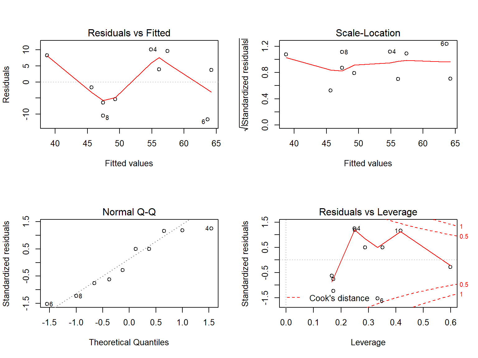
Supplying a model object to the generic plot() function will usually produce a set of regression diagnostics helpful for assessing the assumptions of the regression model.
For lm objects, we get the following plots:
- residual vs fitted
- normal q-q-plot of residuals
- scale-location
- residuals vs leverage
Let’s take a look at these 4 plots for our model. They will not show any strong evidence that the linear regression model is inappropriate.
# plots all 4 plots at once (otherwise one at a time)
layout(matrix(c(1,2,3,4),2,2))

# 4 diagnostic plots
plot(m1)
Inspect the diagnostic plots model m1.
Logistic regression
Logistic regression models how variation in a binary outcome can be explained by a set of predictors.
We can model variation in non-normally distributed outcomes with generalized linear models.
We use glm() for generalized linear models, including logistic regression. Specify the distribution of the outcome in the family= argument. A link function can be specified within family=, but the canonical link function (e.g. link="logit" link for family=binomail) is used as the default, so is not necessary.
Here we model the probability of being insured as predicted by age. The glm() function will model the probability (odds) of insured=1.
# family=binomail uses link=logit by default
m_ins <- glm(insured ~ age, data=bloodtest, family=binomial)
We use the same functions as in linear regression to extract information from our glm model object.
Using summary() on an object of class glm produces a table of regression coefficients again:
summary(m_ins)
##
## Call:
## glm(formula = insured ~ age, family = binomial, data = bloodtest)
##
## Deviance Residuals:
##     Min       1Q   Median       3Q      Max
## -1.8364  -0.6739   0.6244   0.8312   1.1948
##
## Coefficients:
##             Estimate Std. Error z value Pr(>|z|)
## (Intercept) -1.62402    2.75298  -0.590    0.555
## age          0.06089    0.06739   0.904    0.366
##
## (Dispersion parameter for binomial family taken to be 1)
##
##     Null deviance: 12.217  on 9  degrees of freedom
## Residual deviance: 11.339  on 8  degrees of freedom
## AIC: 15.339
##
## Number of Fisher Scoring iterations: 4
Odds ratios for logistic regression are obtained by exponentiating the coefficients and confidence intervals:
# ORs
exp(coef(m2))
##  (Intercept)          age   gendermale  hospitalMDH   hospitalMH
## 7.879529e+09 2.177465e+00 1.241206e+02 1.387734e-04 2.267828e-03

# confidence intervals on ORs
exp(confint(m2))
##                    2.5 %       97.5 %
## (Intercept) 1.843467e-05 3.367946e+24
## age         8.576561e-01 5.528270e+00
## gendermale  2.452115e-06 6.282708e+09
## hospitalMDH 3.162568e-16 6.089375e+07
## hospitalMH  5.916464e-13 8.692766e+06
Graphics
Base R graphics
Base R comes with several powerful graphical functions that give the user a great deal of control over the appearance of the graph.
The graphing functions most commonly used are:
plot(): scatter plotshist(): histogramsboxplot(): box plots (box-and-whisker)barplot(): bar plots
Scatter plots
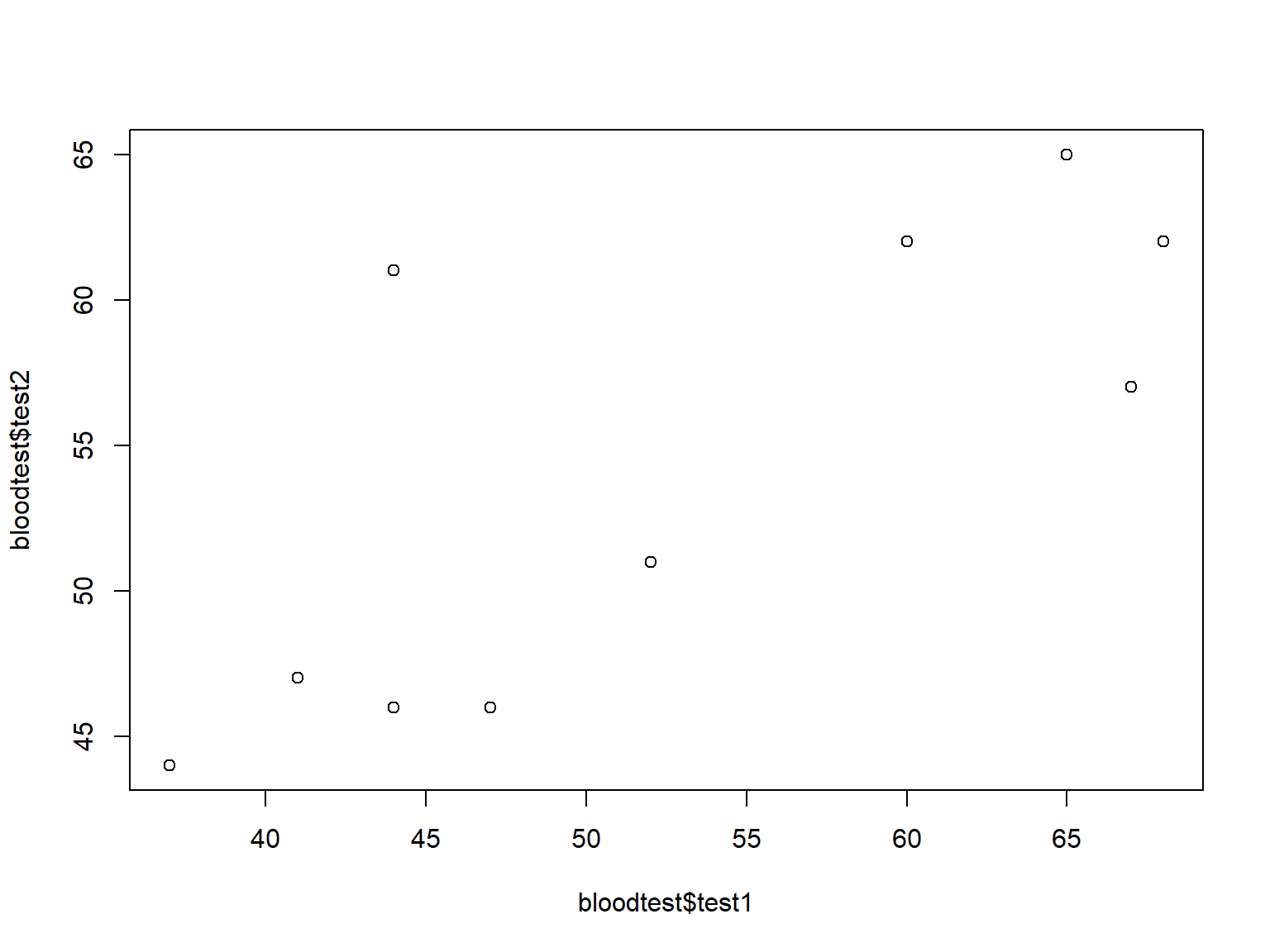
Scatter plots visualize the covariation of two variables, both typically continuous.
Specify two variables to plot() to produce a scatter plot:
plot(bloodtest$test1, bloodtest$test2)
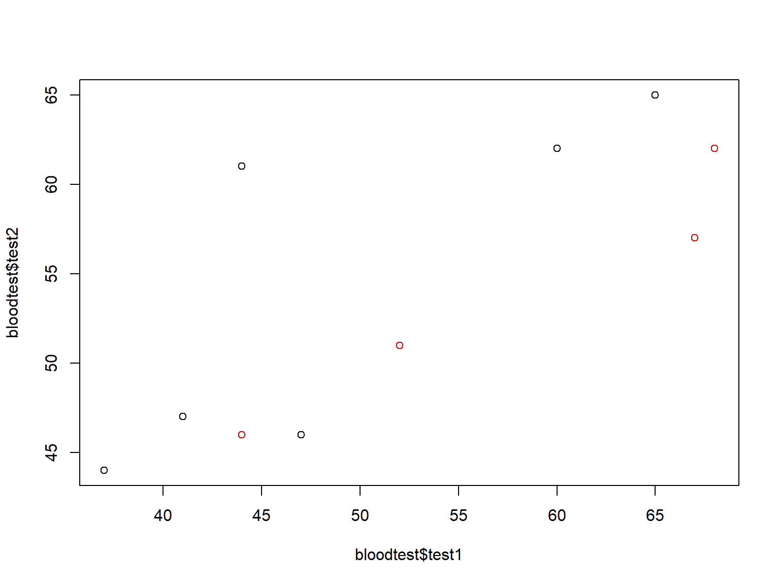
R makes it easy to vary the appearance of graphics by a grouping variable, but the grouping variable must be made into a factor first.
For example, we may want to color the dots by gender with col=:
# factors are categorical variables with numeric codes and string labels
bloodtest$gender <- factor(bloodtest$gender)
plot(bloodtest$test1, bloodtest$test2, col=bloodtest$gender)
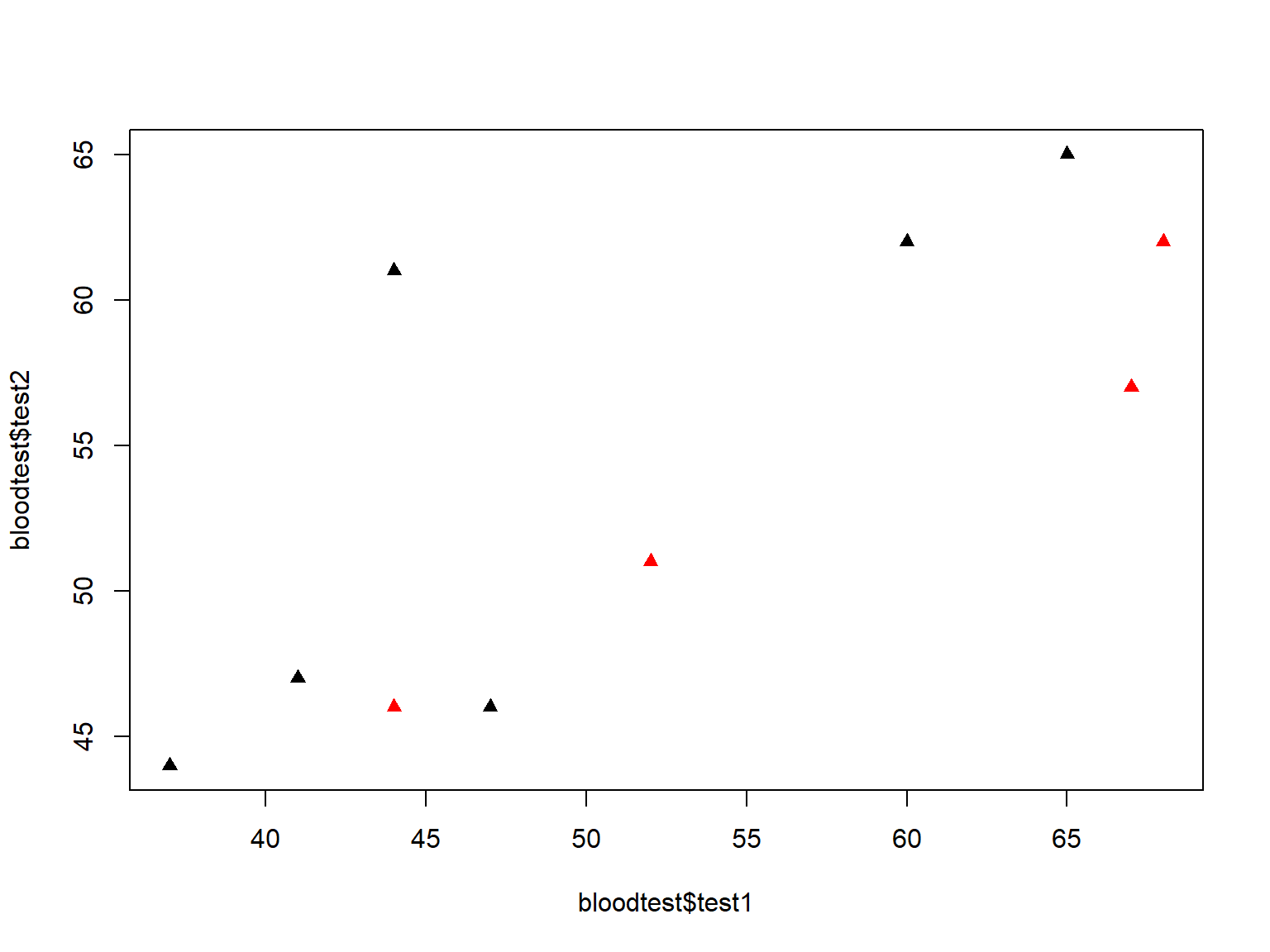
We can change the plotting symbol with pch= (see ?pch for a list of plotting symbols):
plot(bloodtest$test1, bloodtest$test2,
     col=bloodtest$gender,
     pch=17)
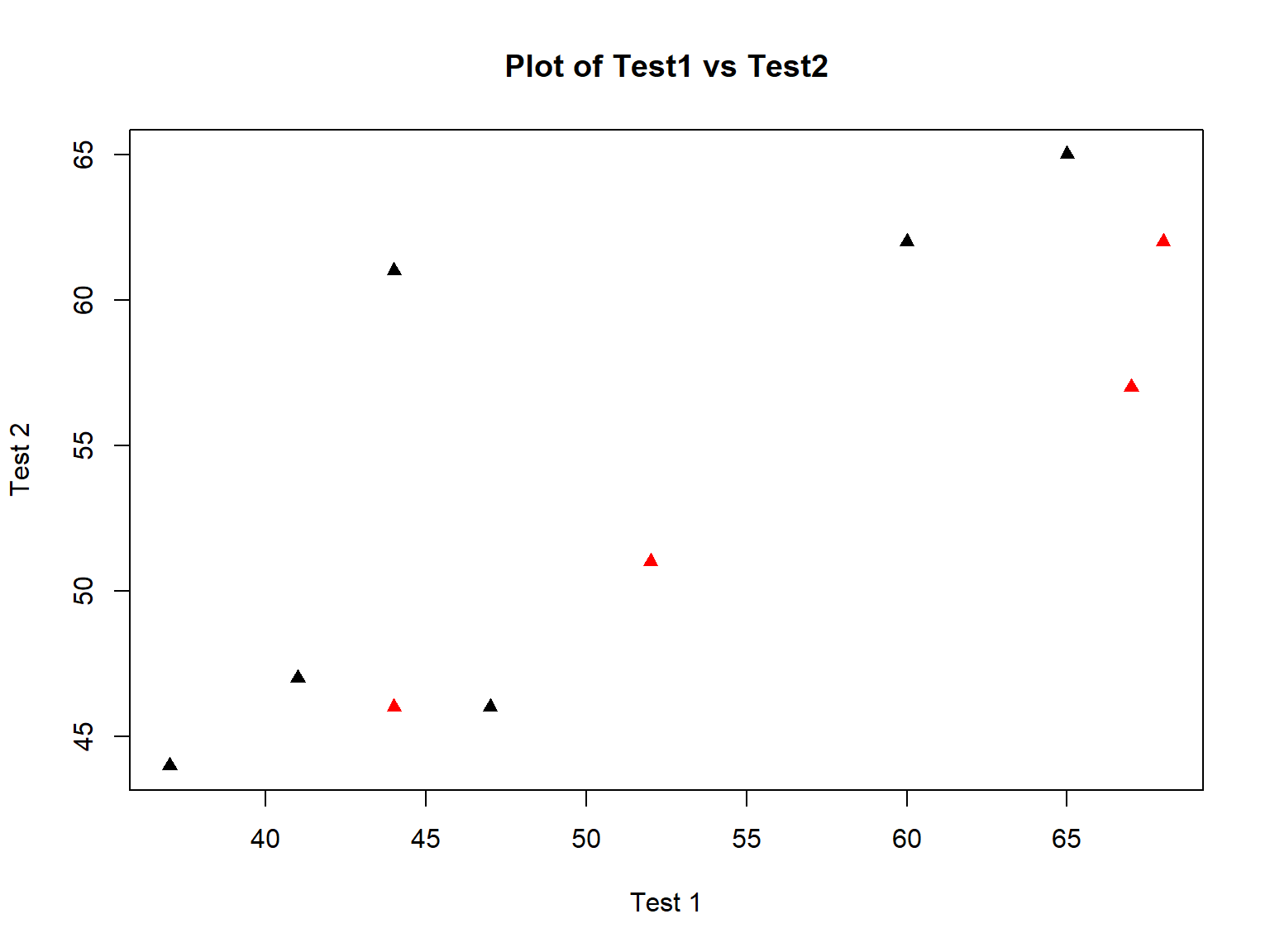
Changing the axis labels and adding a title are easy with xlab=, ylab=, and main=:
plot(bloodtest$test1, bloodtest$test2,
     col=bloodtest$gender,
     pch=17,
     xlab="Test 1",
     ylab="Test 2",
     main="Plot of Test1 vs Test2")
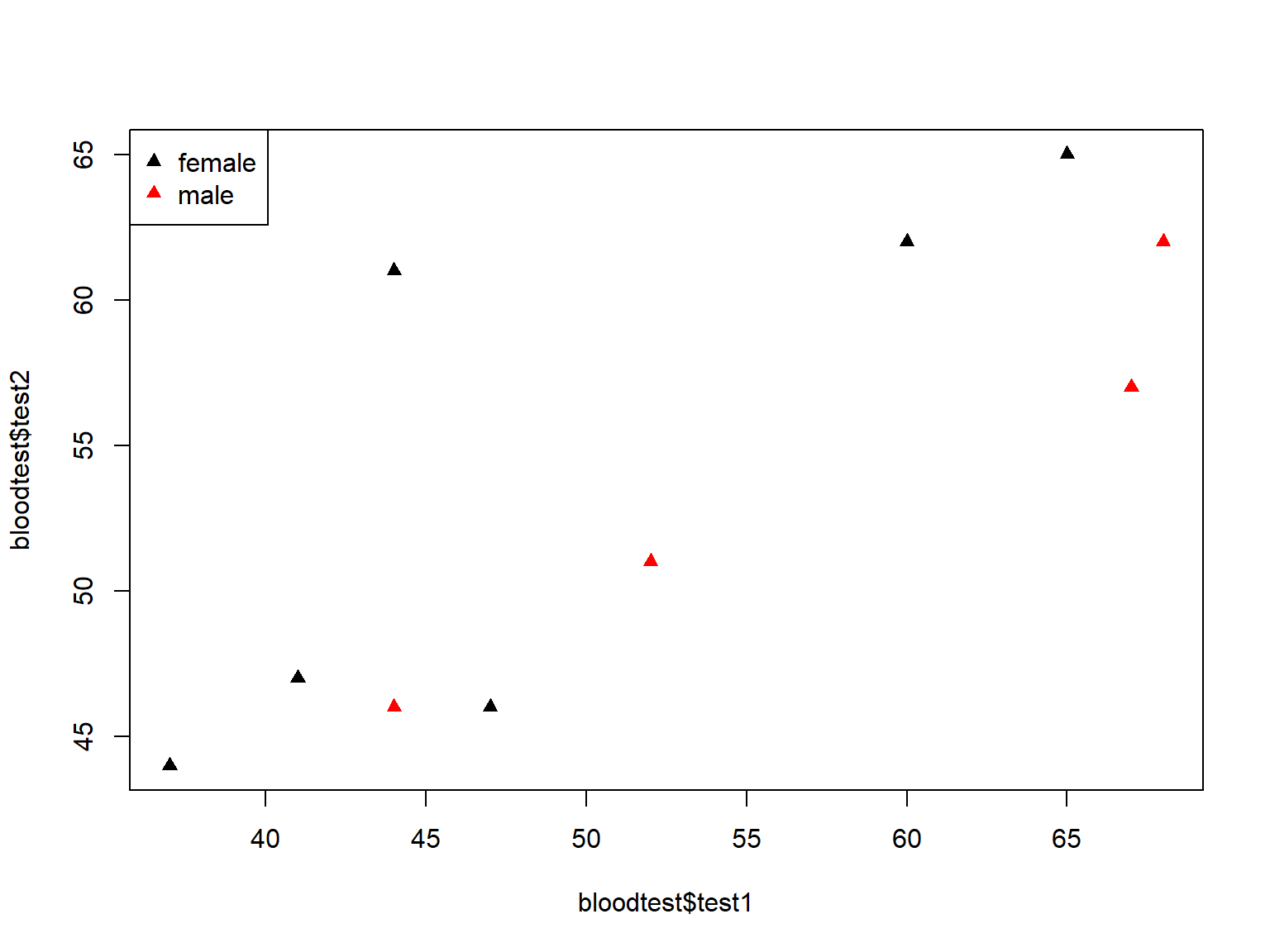
On the other hand, adding a legend to a plot() graph, requires some coding knowledge because you do have a lot of control over its appearance:
plot(bloodtest$test1, bloodtest$test2,
     col=bloodtest$gender,
     pch=17)
# specifies placement, labels, color, and symbol in legend box
legend("topleft", legend=levels(bloodtest$gender), col=c(1:2), pch=17)
Create a scatter plot of read (x-axis) vs write (y-axis), using filled square symbols, colored by the variable prog.
Histograms
Histograms display the distributions of continuous variables.
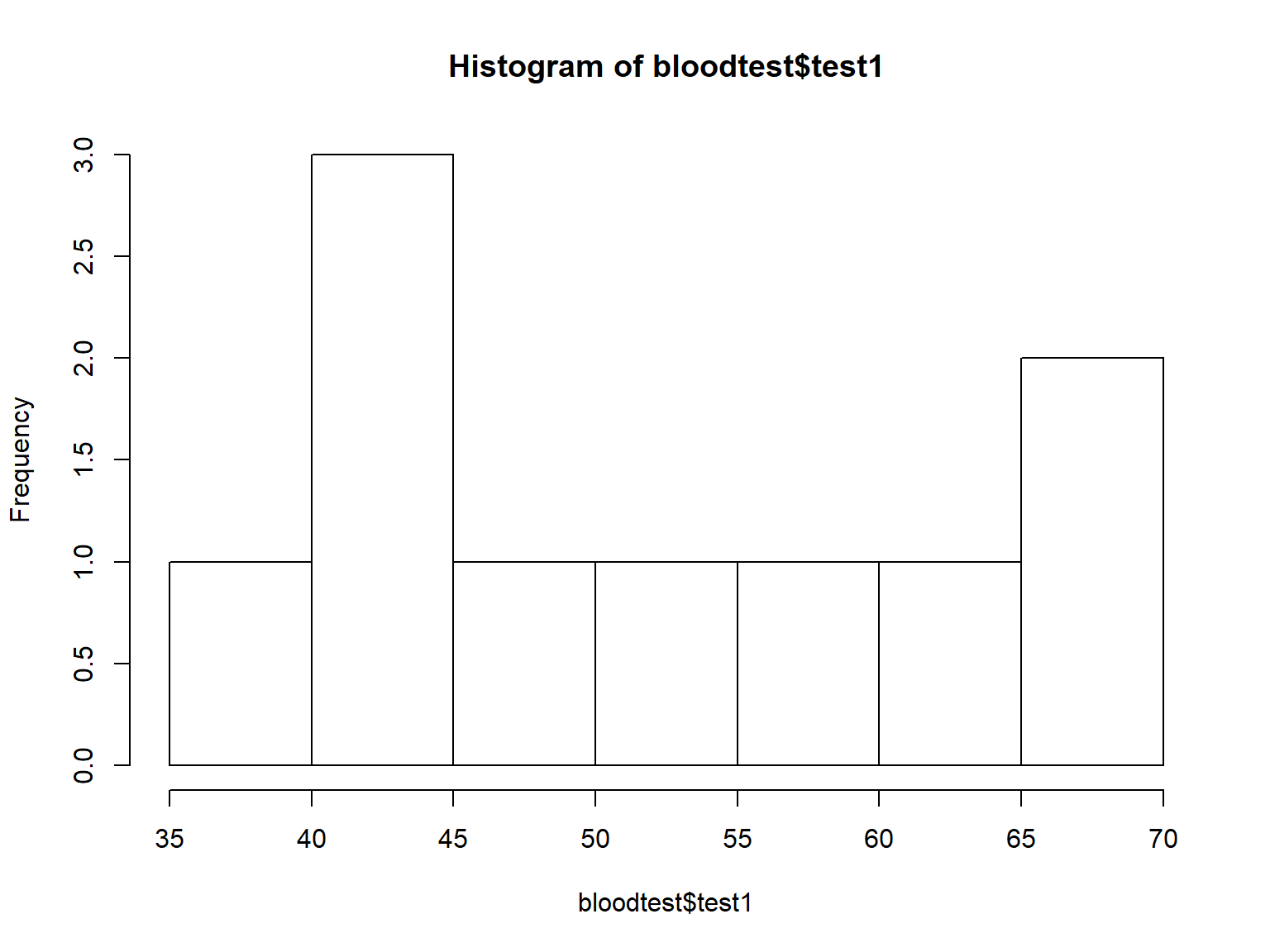
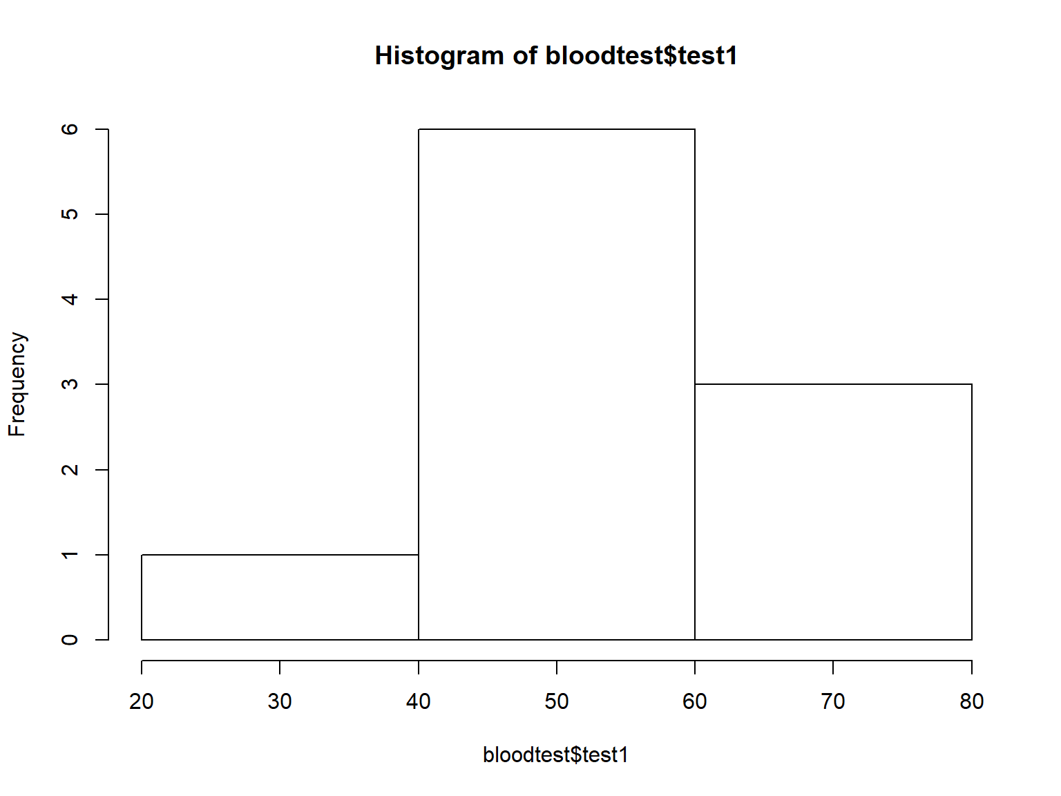
You can adjust the number of bins with the breaks= argument:
hist(bloodtest$test1, breaks=2)
Boxplots
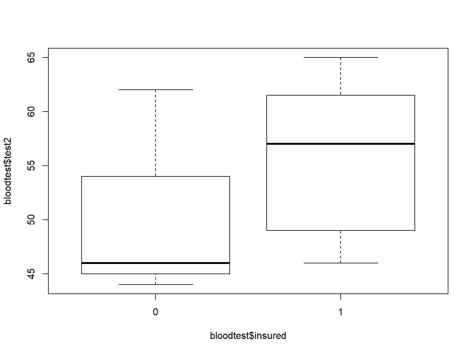
Boxplots are often used to compare the distribution of a continuous variable across the levels of a categorical variable.
Use formula notation in boxplot() to specify boxplots of the variable on the left side of ~ by the variable on the right side.
boxplot(bloodtest$test2 ~ bloodtest$insured)
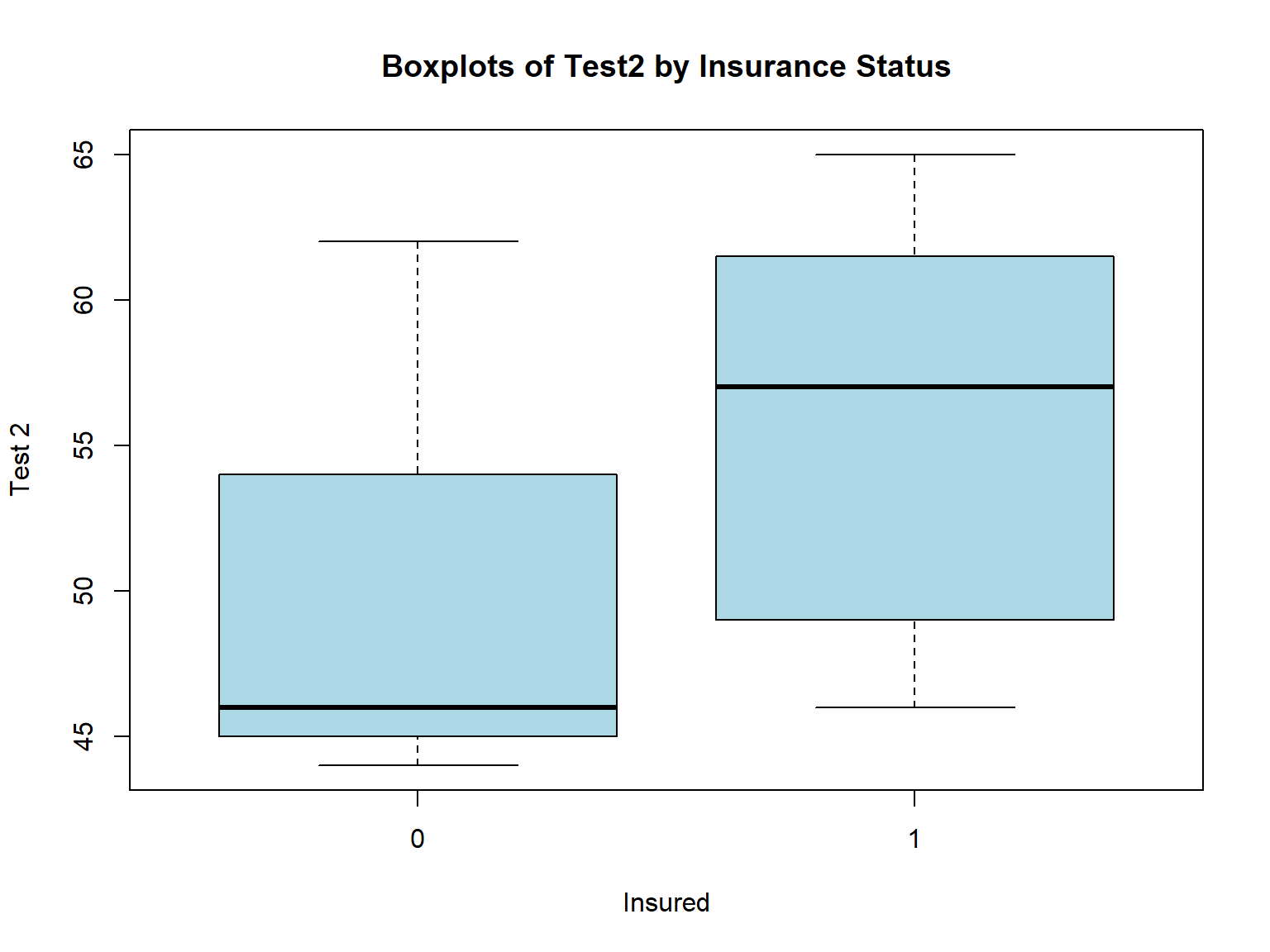
The R plotting functions share many of the same arguments. Here we use xlab=, ylab=, and main= again to change the titles, and col= to change the fill color of the boxes.
boxplot(bloodtest$test2 ~ bloodtest$insured,
        xlab="Insured",
        ylab="Test 2",
        main = "Boxplots of Test2 by Insurance Status",
        col="lightblue")
Barplots
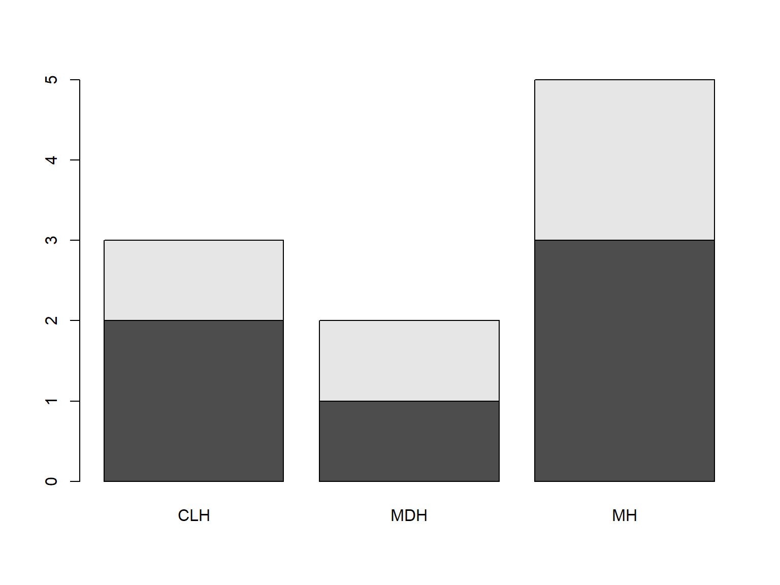
One common use of bar plots is to visualize the frequencies of levels of grouping variables, where the height of the bar represents the number of observations falling into that grouping.
We can thus think of bar plots as graphical representations of frequency tables.
R makes this connection explicit by allowing the output of table() to be used as the input to barplot().
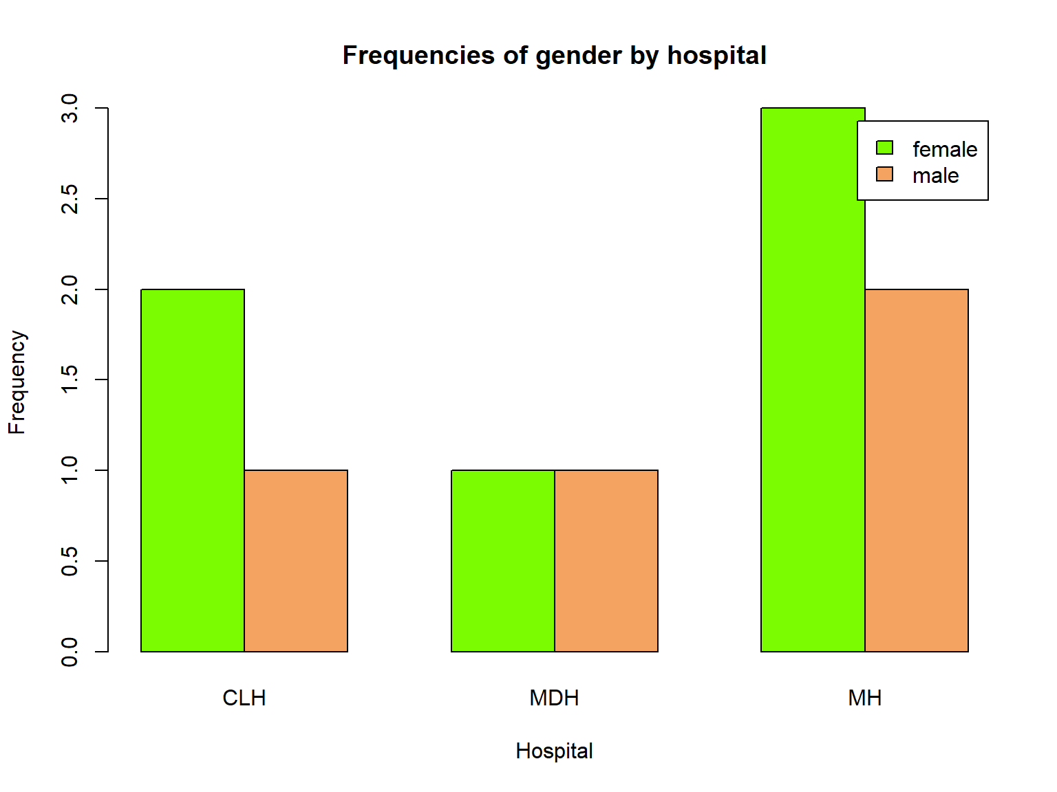
For example, let’s plot the frequencies of groupings made by the variables gender and hospital:
tab <- table(bloodtest$gender, bloodtest$hospital)
barplot(tab)
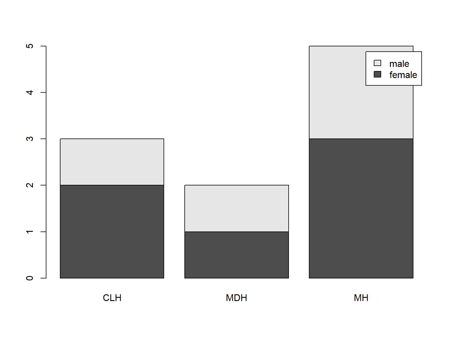
Adding a legend to barplot() is easy (when you use a table as input) with argument legend.text=TRUE:
tab <- table(bloodtest$gender, bloodtest$hospital)
barplot(tab,
        legend.text = TRUE)
Now let’s request side-by-side bars instead of stacked with beside=TRUE:.
We also use col= again to color the bars, but now we have 2 colors to specify, and change our titles as usual:
tab <- table(bloodtest$gender, bloodtest$hospital)
barplot(tab,
        legend.text = TRUE,
        beside=TRUE,
        col=c("lawngreen", "sandybrown"),
        xlab="Hospital",
        ylab="Frequency",
        main="Frequencies of gender by hospital")
Create a bar plot of ses by prog in the data set dat_csv. Use the colors red, green, and blue to color the bars. Add a legend.
Introducing ggplot2 for graphics
Although Base R graphics functions are powerful and can be used to make publication-quality graphics, they are mostly ideal for creating quick, exploratory graphs.
As we saw, adding a legend was somewhat difficult in plot(), and frankly, making the graphs much more complex than what we have shown becomes much more difficult quickly.
The package ggplot2 is a better alternative to create complex, layered, and publication-quality graphics.
ggplot2 uses a structured grammar of graphics that provides an intuitive framework for building graphics layer-by-layer, rather than memorizing lots of plotting commands and optionsggplot2 graphics take less work to make beautiful and eye-catching graphics
Please load the ggplot2 package into your session now with library().
Basic syntax of a ggplot2 plot
The basic specification for a ggplot2 plot is to specify which variables are mapped to which aspects of the graph (called aesthetics) and then to choose a shape (called a geom) to display on the graph.
Although the full syntax of ggplot2 is beyond the scope of this seminar, we can produce many plots with some variation of the following syntax:
ggplot(dataset, aes(x=xvar, y=yvar)) + geom_function()
(Note that the package is named ggplot2 while this function is called ggplot())
That syntax uses the data in dataset, puts xvar on the x-axis, yvar on the y-axis, and uses geom_function() to produce shapes for the graph. For example geom_point() will produce a scatter plot, while geom_boxplot() produces boxplots.
Inside aes(), we can map more variables to graphical aspects of the plot, such as the color, size and shape of plotted objects.
For a much more detailed explanation of the grammar of graphics underlying ggplot2, see our Introduction to ggplot2 seminar.
To demonstrate the graphing capabilities ggplot2 package, we will be using the dat_csv data set.
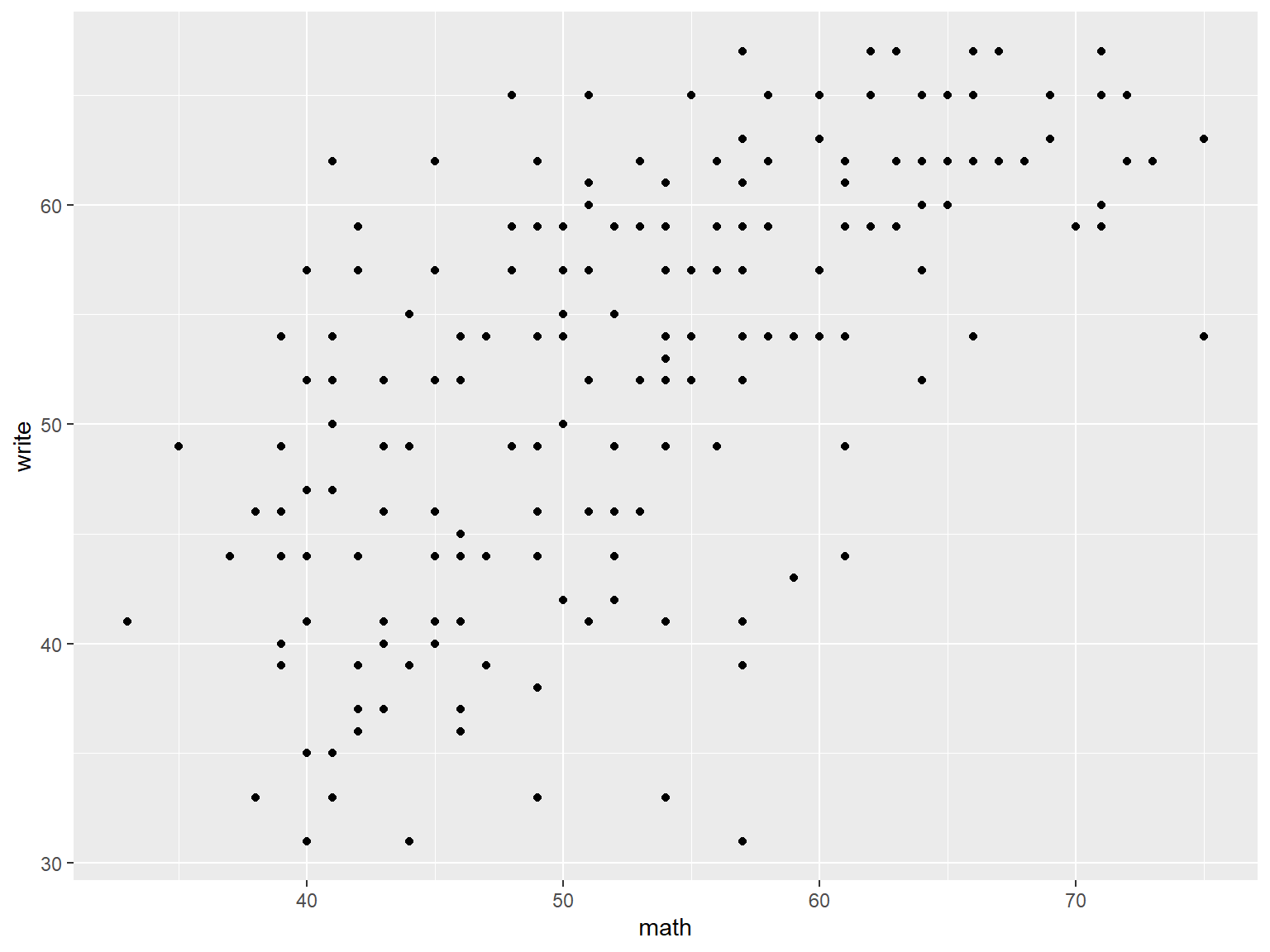
Here we specify a scatter plot of math vs write.
# a scatterplot of math vs write
ggplot(data=dat_csv, aes(x=math, y=write)) +
   geom_point()
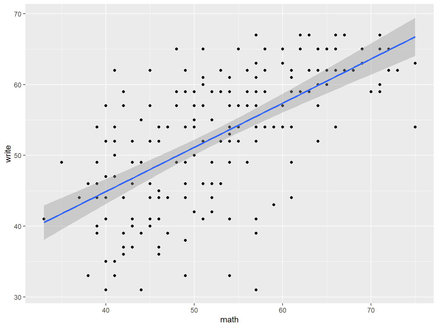
We can add a layer that produces a best-fit regression line (and confidence interval) with geom_smooth().
# a scatterplot of math vs write with best fit line
ggplot(dat_csv, aes(x=math, y=write)) +
  geom_point() +
  geom_smooth(method="lm")
## `geom_smooth()` using formula 'y ~ x'
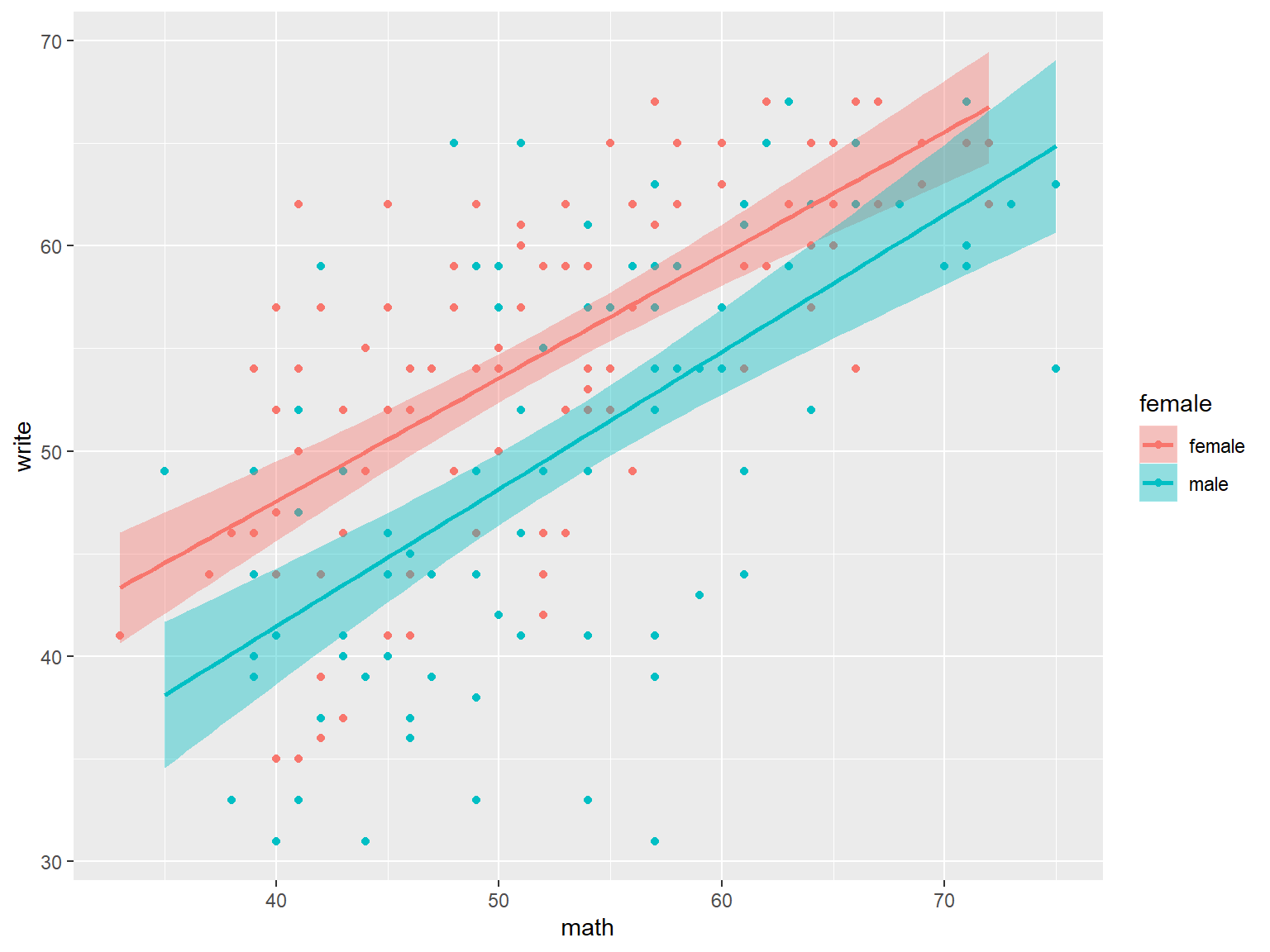
With ggplot, it is easy to link the color, shape, and size of the symbols to a variable.
These aesthetic specifications are used for all geoms. Notice how color and fill will also group the data to produce separate plots.
Also notice that ggplot will insert legends for you by default.
# a scatterplot and best fit line, by gender
#  color affects the best fit line, fill affects the confidence intervals
ggplot(dat_csv, aes(x=math, y=write, color=female, fill=female)) +
  geom_point() +
  geom_smooth(method="lm")
## `geom_smooth()` using formula 'y ~ x'
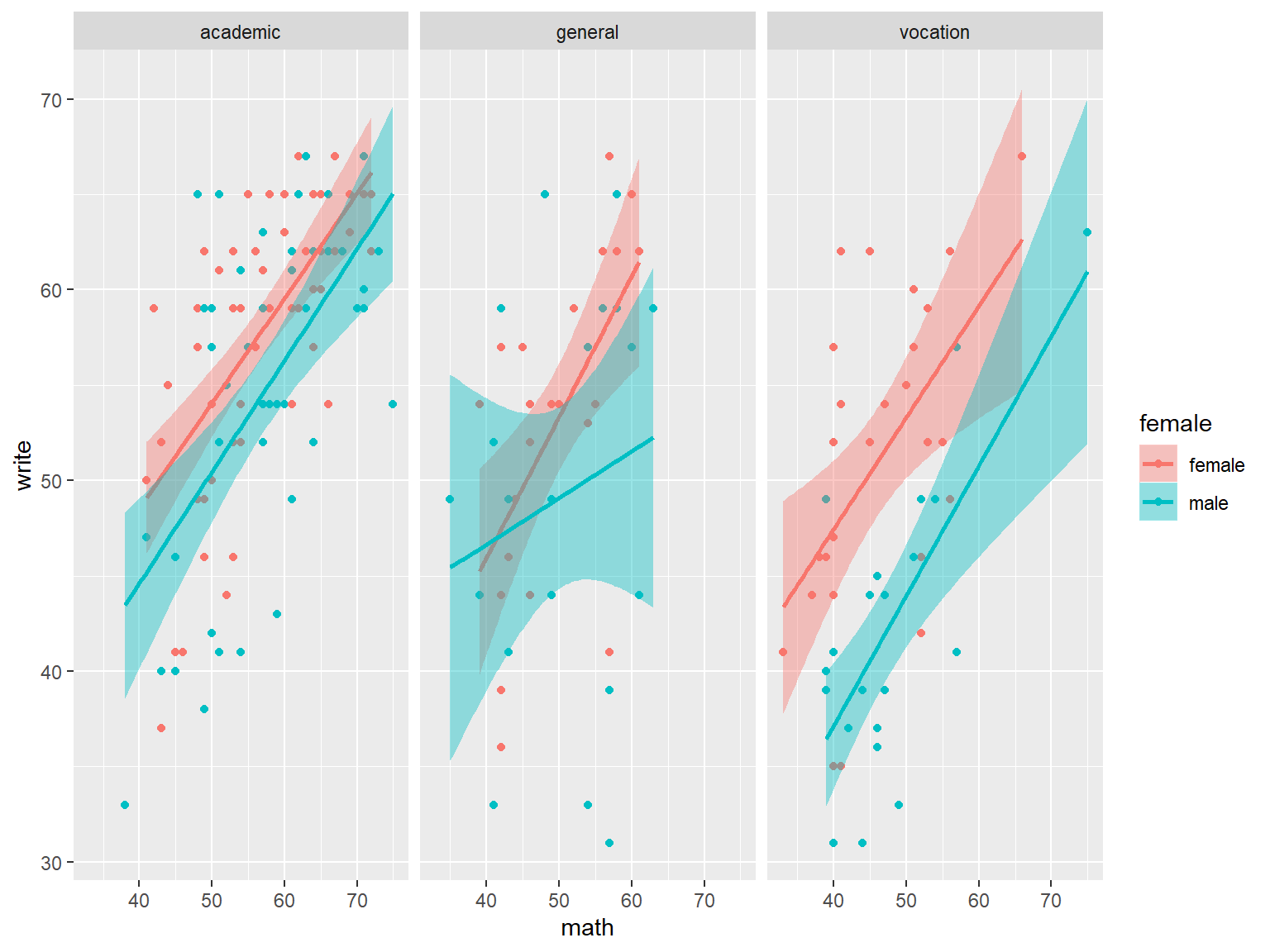
Finally, we can easily make a panel of graphs with the function facet_wrap. Here we create separate plots for each program.
# panel of scatterplot and best fit line, colored by gender, paneled by prog
ggplot(dat_csv, aes(x=math, y=write, color=female, fill=female)) +
  geom_point() +
  geom_smooth(method="lm") +
  facet_wrap(~prog)
## `geom_smooth()` using formula 'y ~ x'
Example 2
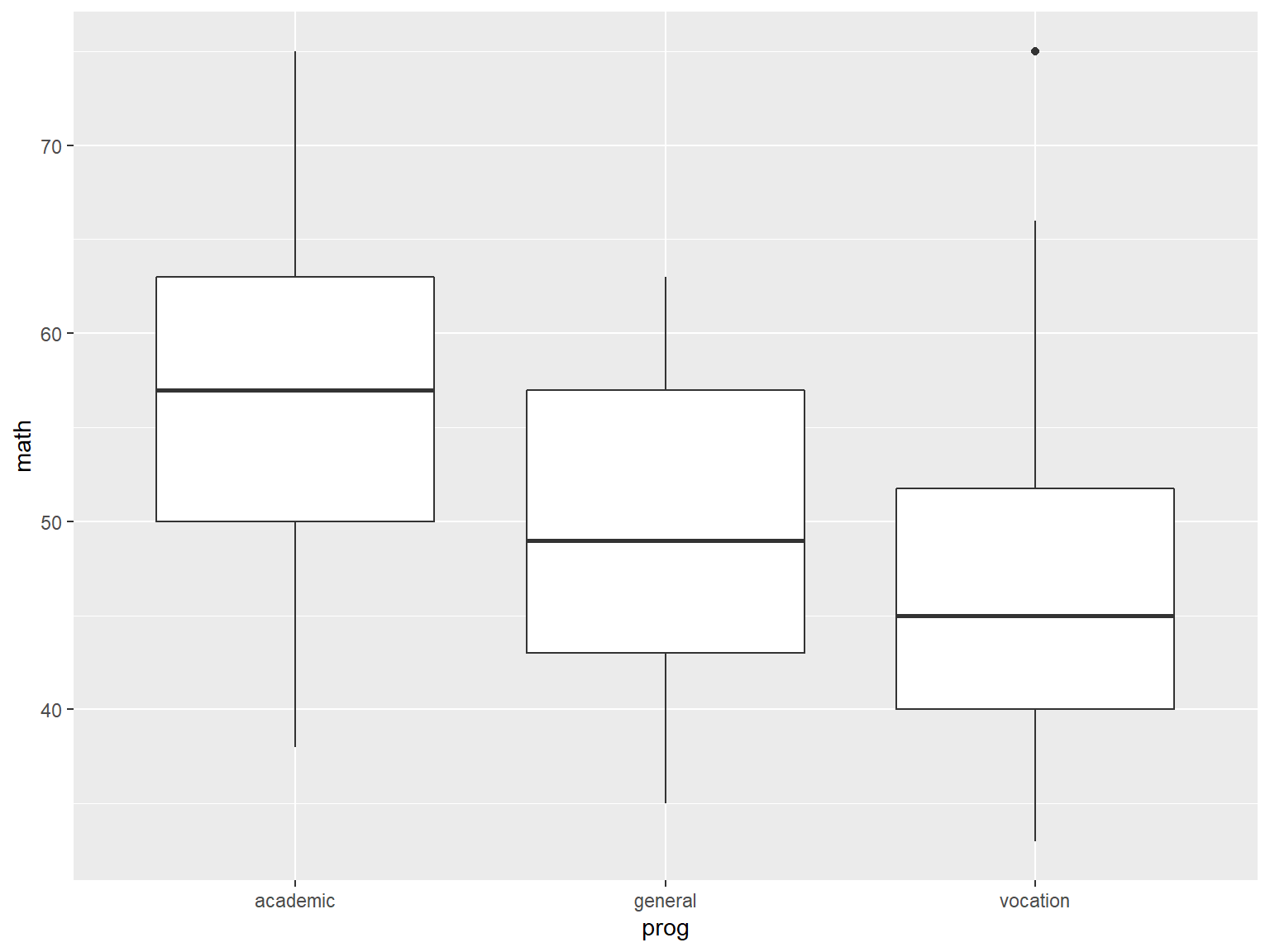
For example 2 of ggplot2 functionality, we start with boxplots of math by prog:
# boxplots of math by prog
ggplot(data=dat_csv, aes(x=prog, y=math)) +
  geom_boxplot()
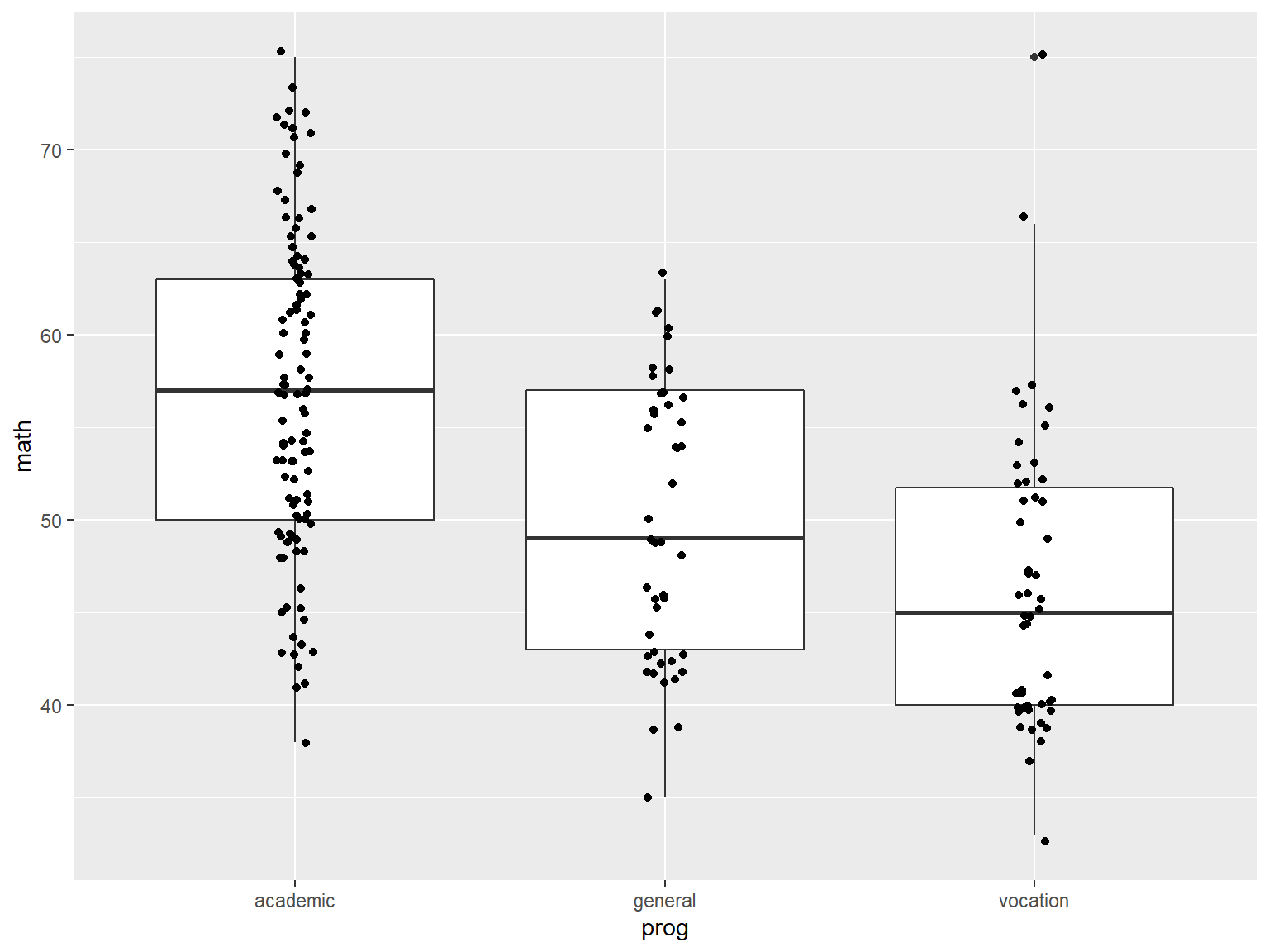
Next we add a layer of jittered data points with geom_jitter() so we can see the actual data (jittering adds a small amount of random variation to the data so that overlapping points will separate):
# boxplots of math by prog, with jittered data points
ggplot(data=dat_csv, aes(x=prog, y=math)) +
  geom_boxplot() +
  geom_jitter(width=.05)
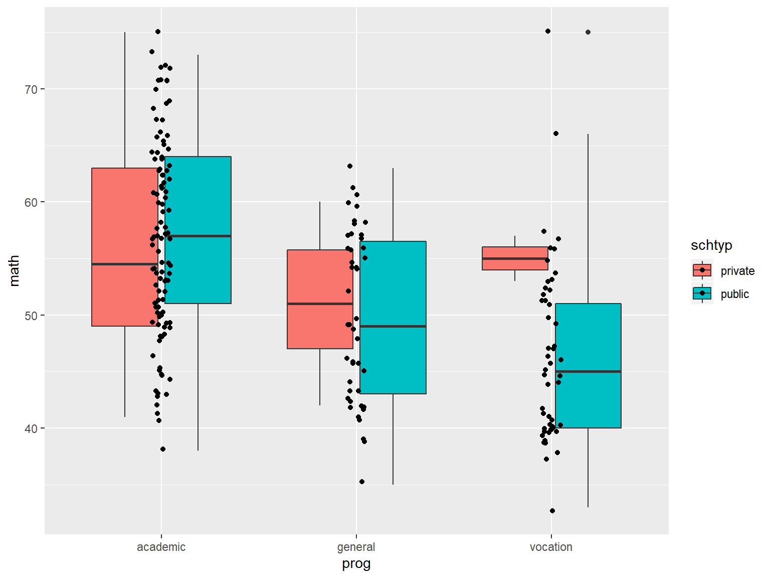
Next we’ll create separate boxplots by school type, by mapping schtyp to fill.
# boxplots of math by prog, with jittered data points
ggplot(data=dat_csv, aes(x=prog, y=math, fill=schtyp)) +
  geom_boxplot() +
  geom_jitter(width=.05)
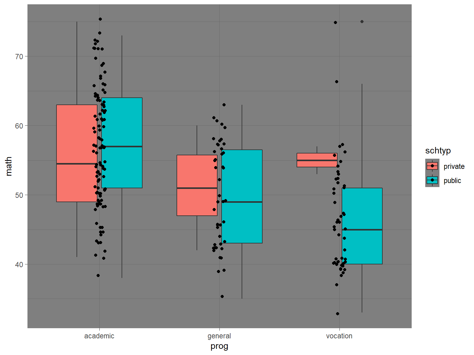
Like base R graphics, you have a great deal of control over the appearance of the graph with ready-made “themes” like theme_dark():
# boxplots of math by prog, with jittered data points, dark theme
ggplot(data=dat_csv, aes(x=prog, y=math, fill=schtyp)) +
  geom_boxplot() +
  geom_jitter(width=.05) +
  theme_dark()
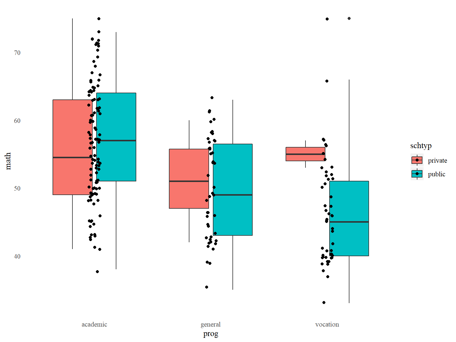
Or you can manually specify everything in theme():
# boxplots of math by prog, with jittered data points, customized appearance
ggplot(data=dat_csv, aes(x=prog, y=math, fill=schtyp)) +
  geom_boxplot() +
  geom_jitter(width=.05) +
  theme(panel.background=element_blank(),  # removes graph background color
        panel.grid=element_blank(),   # removes grid lines
        axis.ticks = element_blank(),   # removes axis ticks
        text=element_text(family="serif"))   # changes font
ggplot2 exercise
Use ggplot2 to make a scatter plot of read (x-axis) vs write (y-axis) from data set dat_csv. Color the dots by ses.
Now add a best fit line with geom_smooth(). Why are there 3 lines?
Sharing your work
RMarkdown
R Markdown allows users to create reproducible documents that weave narrative text together with R code and the output it produces when executed.
One of R Markdown’s great strengths is the variety of output documents it can produce such as HTML webpages, LaTeX documents, and Word documents.
These documents are dynamically generated – whenever we need to change code or data, we can simply update the R Markdown file, compile it, and the output will be automatically updated in the resulting docuemnt.
These documents can then be shared with an audience to provide the most up-to-date content.
For example, this slide-show was entirely produced in R Markdown. When R Markdown encounters the following code block in the file used to create this slide-show, RMarkdown embeds both the code block itself and the output (a graph) into the slide show:
barplot(HairEyeColor[,,1],
        col=c("#4d4d4d", "#bf812d", "#f4a582", "#f6e8c3"),
        legend.text=TRUE, xlab="Eye Color",
        args.legend=list(title="Hair Color"))

R Markdown example
We can open a new Markdown file template through the File menu in RStudio.
A. Choose File -> New File -> R Markdown...
B. Fill the Title field and Author fields with “Practice” and your name, respectively.
C. In the left menu, select Document, and for Default Output Format select option HTML (these are the defaults).
D. Click OK
R Markdown files typically use the extension .Rmd or .rmd
R Markdown files consist of 3 elements:
- YAML header: The header between
--- at the top; determines document type and overall appearance
- Markdown: code tags like
## and ** used to format text
- R code chunks: delineated by ``` and used to process data and output results
Once we are pleased with its contents, we can compile the R Markdown file and render it into its final output format by clicking the Knit button.
Click the Knit button on your R Markdown document. Save the file with the name myfirst.rmd. Observe how each element in the R Markdown file becomes an element in the output document. Note: If R tells you that you need to install some packages before knitting, you must install the packages for R to output the documents.
Markdown
Markdown is a lightweight markup language, which is a system of code tags used to format documents. Tags are used to define sections, change the appearance of text, build tables, link images, and so on.
Hypertext Markup Language (HTML) is a markup language designed to be used for web pages. The placement and appearance of text, images, frames, tables, and other elements can all be specified in HTML.
Markdown was originally designed to be a shorthand for HTML. For example in HTML, to italicize text, you enclose it in <em> </em>. In Markdown, you just enclose it in * *.
Some important Markdown tags:
*italics* produces italics**bold** produces bold~~strikethrough~~ produces strikethrough`code` produces codetext^super^ produces textsupertext~sub~ produces textsub
Do not insert spaces in between formatting tags and the text.
Identify which text in your .rmd file has been formatted with Markdown tags.
Try changing the bolded word to italics.
The Markdown tag # is used for section header. To treat text as a header, place one to six # tags at the beginning of the header text. The number of # signs indicate the level of the header (higher levels will be displayed in larger fonts).
Headers should be preceded by a blank line, and there should be a space between the # tags and the header text
Add a level 4 header to the document called “Header 4”, knit the document, and compare its size to the other 2 headers.
R Code chunks
For R Markdown files, R code is placed in code chunks that can be interleaved with the text of the document. All of the code chunks execute sequentially in one session when the .rmd file is rendered, so objects created in one chunk are available to all subsequent chunks.
R Markdown actually uses the package knitr to process the R code chunks.
A large array of knitr options allows some control over the appearance of R code, text output and graphical output in the final document.
R code chunks are delimited by ```{r chunk_label, options} at the beginning and ``` at the end. The chunk_label and options are indeed optional and are separated by commas (much more on this soon). You can type out the tags, or use the shortcut Ctrl + Alt + I (Cmd + Option + I on Macs), or use the Insert button at the top right of the script editor (will appear if the file extension is .rmd).
Add an R code chunk using the keyboard shortcut or the Insert button to your R Markdown file. Inside the chunk, create a histogram of the variable speed in the data set cars that is automatically loaded with R.
Code chunk options
R Markdown (via knitr) allows a great deal of control over R code chunk output via the knitr chunk options.
For example, we can suppress the output histogram with the option eval=FALSE and suppress printing of the code chunk with echo=FALSE. Place the option in the chunk header, inside ```{r }.
Add eval=FALSE to the chunk you just created and observe the results.
Now add echo=FALSE to the same chunk, separated by a comma.
knitr provides many options to control the appearance of graphics, with options like fig.width= and fig.height=.
Remove eval=FALSE and echo=FALSE from your latest chunk. Add fig.width=3, separated by a comma, and observe the results.
Shiny
The shiny package is used to create interactive apps as webpages or even embedded in an RMarkdown document.
With shiny, you program the code for a graphical interface that allows the user to harness R’s data visualization and analysis tools to interact with data.
You will need a computer actively running R to use the app:
Fortunately, creation of web apps with shiny does not require advanced web programming skills.
Learning the syntax of a shiny app is beyond the scope of this presentation, but we can see its potential with a few of the example apps that come with the pacakage.
Load the shiny library into your current R session with library().
Shiny example 1
The first and simplest shiny example demonstrates the interactivity of a shiny app:
Issue runExample("01_hello") in the RStudio console
Move the slider back and forth and observe how the graph changes reactively with user input.
At the bottom of the app, we see the code used to generate the app.
While you are running a shiny app in an R session, you will not be able to use R. To close the app and enable R to be used, hit Esc, click the stop sign in the RStudio console, or use the X at the top right of the app interface.
Shiny example 2
The second example features a more complex app with tabs.
Issue runExample("06_tabsets") in the RStudio console
Each tab runs a different function on the (randomly-generated) data, the first runs hist(), the second summary(), and the third print() (implicitly).
The example also features radio-button inputs
Shiny example 3
OUr third example showcases shiny’s wide-ranging functionality.
Issue runExample("10_download") in the RStudio console.
With shiny running on a dedicated server, users can download your data or whatever objects you make available.
For more inspiration take a look at some publicly available apps at the Shiny Gallery.
More help
UCLA IDRE Seminars
- R Data Management
- R Markdown
- R graphics with ggplot2
- Linear regression in R
Getting help online
- UCLA Stat Consulting, our website with thousands of pages for help with statistical analysis
- StackOverflow, a message board where R-related and statistics-related questions are answered
- R for Data Science, an online book written by the people who make RStudio and the tidyverse, that discusses how to use R for all steps of data analysis, with special emphasis on using the tidyverse
Thank you!


