Function interaction.plot can be used to make spaghetti plots. Let’s use data set
tolerance_pp.csv used in Applied Longitudinal Data Analysis: Modeling Change and Event Occurrence
by Judith D. Singer and John B. Willett for our example.
tolerance<-read.table("https://stats.idre.ucla.edu/stat/r/faq/tolpp.csv",
sep=",", header=T)
head(tolerance, n=10)

   id age tolerance male exposure time
1   9  11      2.23    0     1.54    0
2   9  12      1.79    0     1.54    1
3   9  13      1.90    0     1.54    2
4   9  14      2.12    0     1.54    3
5   9  15      2.66    0     1.54    4
6  45  11      1.12    1     1.16    0
7  45  12      1.45    1     1.16    1
8  45  13      1.45    1     1.16    2
9  45  14      1.45    1     1.16    3
10 45  15      1.99    1     1.16    4
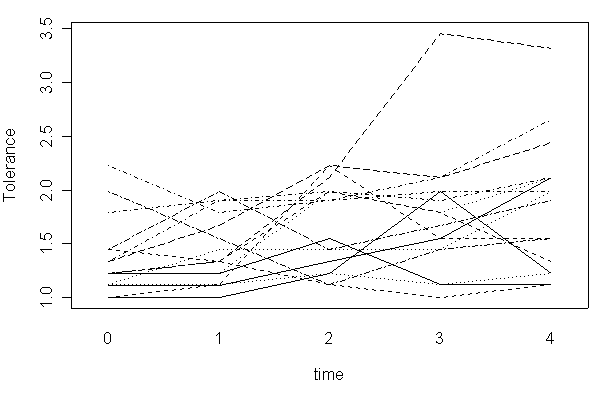
Each subject has been observed at five time points. We will plot the outcome variable tolerance
against time for each subject.
interaction.plot(tolerance$time,
tolerance$id, tolerance$tolerance, xlab="time", ylab="Tolerance", legend=F)
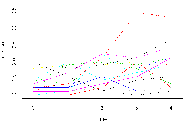
We can also use different colors for different lines.
interaction.plot(tolerance$time,
tolerance$id, tolerance$tolerance,
xlab="time", ylab="Tolerance", col=c(1:10), legend=F)
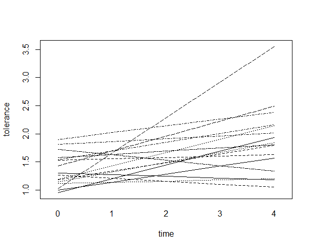
Here is a more involved example. We will make a spaghetti plot of linear trend for each subject.
First we create an object of fitted values for each subject. The function by is quite handy for this
type of task. The first argument is the entire data set, the second argument is the group id variable (the
by variable), and the third argument is the function to apply to each group. Here we define the function
on-the-fly to be the fitted value from the linear regression of variable tolerance on time. Each value of
variable id yields a sub data set for the regression function and this has to be the argument for this function.
The function unlist converts the list object fit into a vector object and we will have to get rid
of the names for it by assign NULL to its names.
#fitting the linear model by id
fit <- by(tolerance, tolerance$id,
       function(x) fitted.values(lm(tolerance ~
time, data=x)))

fit1 <- unlist(fit)
names(fit1) <- NULL
#plotting the linear fit by id
interaction.plot(tolerance$time, tolerance$id, fit1,
xlab="time", ylab="tolerance", legend=F)