
1. Plotting Devices
2. Graph Functions
3. Parameter Settings
4. Exporting Graphs
Plotting Devices:
If you are working on a windows platform then when you use a function which
creates a graph a graphics window will automatically be launched. Common device functions include: dev.off, dev.set, graphics.off. These functions
are especially useful if there is more than one graphics window open. Only one device can
be active and it is in the active device that all the graphics operations occur. The function
dev.set is used to specify which device is going to be active. The output from the dev.set
function is to list the number of the active device.
The dev.off function is used to close a specific device. The default of dev.off is to
close the current device. The function graphics.off will close all the devices at once.
Graph functions
Common functions to create plots: plot, boxplot, barplot, stars, pairs,
matplot, hist, image, contour.
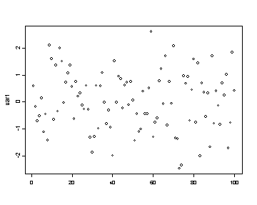
In order to see the specifics for each function please consult the help pages. The plot function is the most basic plotting function.
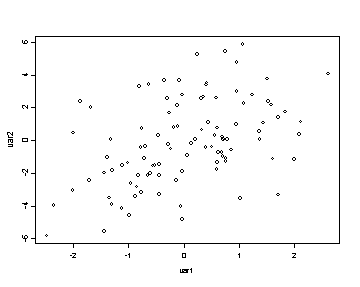
Using the plot function with only one variable will result in an index plot. Using two variables in the plot function will result in a
graph with the first argument as the variable plotted on the x-axis and the second
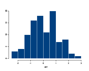
argument as the variable plotted on the y-axis. In the following example we create two variables, var1 and var2,
and graph them using the plot and hist functions.
var1 <- rnorm(100)
plot(var1)
var2 <- var1 + 2*rnorm(100)
plot(var1, var2)
hist(var1)
Common functions that will add features to an existing plot: points, lines, text,
mtext, image, contour, title, legend. This
is not the exhaustive list of all the functions that will add to a plot
since this list would be too long to include here. Furthermore, to understand the specific
features of each function please consult the help pages. Note that image and contour
can be used to add to an existing plot by using the option add and setting it to TRUE.
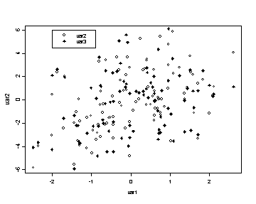
In the following example we graph two variables using the points function and we
identify the two variables using the legend function. The pch option in the
points function changes the symbols used in the plot. Basic marks are
device-dependent, but generally adhere to the following standards: square (0);
circle (or octagon) (1); triangle (2); cross (3); X (4); diamond (5) and
inverted triangle (6). To get superimposed versions of the above use the
following arithmetic(!): 7=0+4; 8=3+4; 9=3+5; 10=1+3; 11=2+6; 12=0+3; 13=1+4;
14=0+2. Filled marks are square (15), octagon (16), triangle (17), and diamond
(18). Using the numbers 32 through 126 for pch
yields the 95 ASCII characters from space through tilde (see the S-PLUS data set
font). The numbers between 161 and 252 yield characters,
accents, ligatures, or nothing, depending on the font (which is device
dependent). In the legend function the first
argument is the x-coordinate of the upper right hand corner of the legend box, the
second argument is the y-coordinate, the third argument is the list of the text
to be displayed and the marks option specifies which symbols will be displayed.
plot(var1, var2)
var3 <- var2 + 2*rnorm(100)
points(var1, var3, pch=18)
legend(-2, 6, c("var2", "var3"), marks= c(1, 18) )
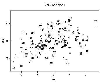
The next example uses the plot, text and title functions. The
text function allows you to label points in the graph. The default option
is to display the observation number for each point. The option ylim
determines the limits of the y-axis.
plot(var1, var2, ylim = c(-8, 8))
text(var1, var3)
title( "var2 and var3")
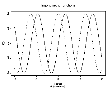
The next graph will illustrate the use of the function lines to add lines to an existing graph.
The type option in the plot function is used to specify which type of graph to be plotted including points (“p”),
lines (“l”), vertical height bars (“h”), and step-functions (“s”). The xlab and
ylab options in the plot function change the labels on the x and y-axes respectively. The lines types used in the
graph can be changed by using the lty option. The title function will place the first argument as a title
above the graph and the second argument as a title below the graph.
x <- seq( -10, 10, length = 1000)
plot(x, sin(x), xlab="x-values", ylab="f(x)", type="l")
lines(x, cos(x), lty=3)
title( "Trigonometric functions", "sin(x) and cos(x)")
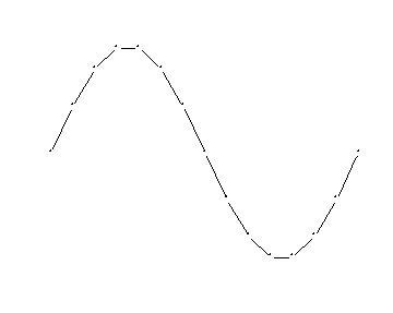
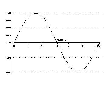
The following example illustrates how you can build a graph in R. We start by using the plot function
but this time we use the axes option to indicate that we do not want to utilize the default axes.
We use the pch option to change the symbols used in the graph.
We want to show both the symbols at each point plotted and draw a line connecting the points, so we use the type option to
plot both lines and symbols.
x <- seq( 0, 2*pi, length = 15)
y <- sin(x)
plot(x, y, axes=F, type="b", pch="*", xlab=" ", ylab=" ")
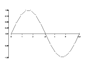
Now we would like to add axes to the graph and we do this using the axis function.
axis ( 1, at = c(0, 1, 2, pi, 4, 5, 2*pi), labels = c(0, 1, 2, "pi", 4, 5, "2 pi"), pos=0)
axis (2, at = c( -1, -0.5, 0, 0.25, 0.5, 0.75, 1) )
Finally, we want to add the reference lines and the text at the coordinates (pi, 0). The
abline function
adds lines to the graph and when using the h options we indicate that we want the lines to be horizontal reference
lines and thus we only need to specify the y-intercept for each line. The adj option in the text function
determines how the text is adjusted (0=left justified, .5=centered, and 1=right justified).
abline( h= c(-1, -0.5, 0.5, 1), lty=2)
text( pi, 0.1, "sin(pi) = 0", adj=0)
Parameter Settings:
It is possible to set the parameters of the graphs globally by using the par function. However, if
the graphs being produced vary from graph to graph then it is probably more useful to set the parameters
within each plotting function. The most commonly used parameter settings
include mfrow (multiple figures by row) and mfcol (multiple
figures by column) which determine the layout of multiple graphs in one graphing
device. By specifying mfrow = c(n,m) the results will be an n*m
matrix of graphs that are filled by rows, using the mfcol option would
generate the same graphics layout but it would be filled by columns rather than
by rows. The placement of the graph within the graphics device is determine by
fig=c(x1,x2,y1,y2) where x1-y2 are the coordinates of the current figure region expressed as a fraction of
the device surface. This is dependent on mfrow and mfcol.
Margins size in inches are determined by mai=c(xbot,xlef,xtop,xrig).
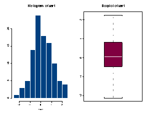
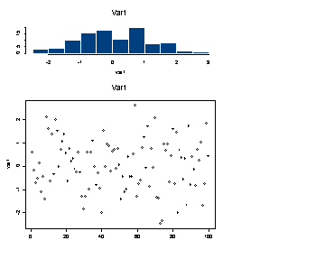
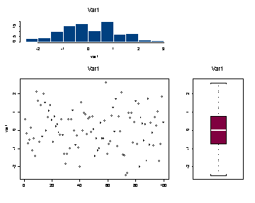
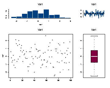
The first example illustrates the use of the option mfcol and the second
example illustrates the use of the fig option for including multiple
plots in one frame. In the second example the function frame clears any graphs from
the current device.
par( mfcol= c(1, 2))
hist(var1)
title( "Histogram of var1")
boxplot(var1)
title("Boxplot of var1")
frame()
par( fig = c( 0, .7, 0 , .7) )
plot(var1)
title( "Var1")
par( fig = c(0, .7, .7, 1) )
hist(var1)
title( "Var1")
par( fig = c(.7, 1, 0, .7))
boxplot(var1)
title( "Var1")
par( fig = c(.7, 1, .7, 1) )
barplot(var1)
title( "Var1")
Exporting Graphs:
It is possibly to save graphs created in SPLUS in many different formats using the export.graph
function. These formats including the ever popular postscript (ps), portable networks graphics (png),
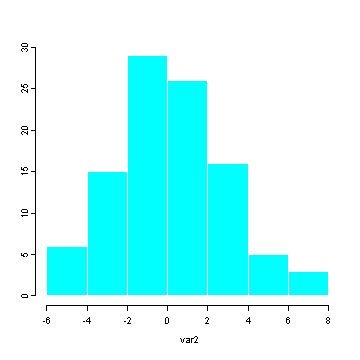
windows bitmap (bmp), gif and jpeg. The following is an example of exporting a histogram as a png format
that is 5 inches high and 6 inches wide and then as a jpeg which is 10 cm high and 12 centimeters wide.
Note that Name is a required argument which indicates from which device you
are obtaining the graph. In this example we are using the default device which is GSD2.
Furthermore, the argument Name must be capitalized whereas the other arguments can be
either upper or lower case.
hist(var1)
export.graph("C:temphttps://stats.idre.ucla.edu/wp-content/uploads/2016/02/hist1.png", Name="GSD2", exporttype = "PNG", height=5, width=6)
hist(var2)
export.graph("C:temphttps://stats.idre.ucla.edu/wp-content/uploads/2016/02/hist2.jpg", Name="GSD2", exporttype = "JPG", height=13,
              width=15, units="cm")
The postscript file can also be generated using the postscript function.
The following example show how to save a histogram of var1 as a postscript file using the
postscript function.
postscript("hist.ps")
hist(var1)
dev.off()
These graphs can be created by using the export graph menu located
under the File menu.
The following example shows how to save an SPLUS graph as a portable network graphics file using
the export menu. The export graph menu will only be available if the currently active
device is the graph device.
FILE
 EXPORT GRAPH
  Select the file type (in this case Portable Network Graphics (PNG)) and
  browse to the folder where the file will be saved to.