
Version info: Code for this page was tested in SAS 9.3.
Exact logistic regression is used to model binary outcome variables in which the
log odds of the outcome is modeled as a linear combination of the predictor
variables. It is used when the sample size is too small for a regular
logistic regression (which uses the standard maximum-likelihood-based estimator) and/or when some of the cells formed by the outcome and
categorical predictor variable have no observations. The estimates given
by exact logistic regression do not depend on asymptotic results.
Please note: The purpose of this page is to show how to use various data
analysis commands. It does not cover all aspects of the research process which
researchers are expected to do. In particular, it does not cover data
cleaning and checking, verification of assumptions, model diagnostics or
potential follow-up analyses.
Example
Suppose that we are interested in the factors
that influence whether or not a high school senior is admitted into a very competitive
engineering school. The
outcome variable is binary (0/1): admit or not admit.
The predictor variables of interest include student gender and whether or not the
student took Advanced Placement calculus in high school. Because the response variable is binary, we need
to use a model that handles 0/1 outcome variables correctly. Also, because of the number of students
involved is small, we will need a procedure that can perform the estimation with
a small sample size.
Description of the data
The data for this exact logistic data analysis include the number of students admitted, the total
number of applicants broken down by gender (the variable female), and whether or not
they had taken AP calculus (the variable apcalc). Since the dataset
is so small, we will read it in directly.
options nocenter;

data exlogit;
  input female apcalc admit num;
datalines;
0 0 0 7
0 0 1 1
0 1 0 3
0 1 1 7
1 0 0 5
1 0 1 1
1 1 0 0
1 1 1 6
;
run;
Let’s look at some frequency tables. We will specify the variable num
as the frequency weight.
proc freq data = exlogit;
  tables female*(apcalc admit);
  tables apcalc*admit;
  weight num;
run;

Table of female by apcalc

female     apcalc

Frequency|
Percent  |
Row Pct  |
Col Pct  |       0|       1|  Total
---------+--------+--------+
       0 |      8 |     10 |     18
         |  26.67 |  33.33 |  60.00
         |  44.44 |  55.56 |
         |  57.14 |  62.50 |
---------+--------+--------+
       1 |      6 |      6 |     12
         |  20.00 |  20.00 |  40.00
         |  50.00 |  50.00 |
         |  42.86 |  37.50 |
---------+--------+--------+
Total          14       16       30
            46.67    53.33   100.00

Table of female by admit

female     admit

Frequency|
Percent  |
Row Pct  |
Col Pct  |       0|       1|  Total
---------+--------+--------+
       0 |     10 |      8 |     18
         |  33.33 |  26.67 |  60.00
         |  55.56 |  44.44 |
         |  66.67 |  53.33 |
---------+--------+--------+
       1 |      5 |      7 |     12
         |  16.67 |  23.33 |  40.00
         |  41.67 |  58.33 |
         |  33.33 |  46.67 |
---------+--------+--------+
Total          15       15       30
            50.00    50.00   100.00

Table of apcalc by admit

apcalc     admit

Frequency|
Percent  |
Row Pct  |
Col Pct  |       0|       1|  Total
---------+--------+--------+
       0 |     12 |      2 |     14
         |  40.00 |   6.67 |  46.67
         |  85.71 |  14.29 |
         |  80.00 |  13.33 |
---------+--------+--------+
       1 |      3 |     13 |     16
         |  10.00 |  43.33 |  53.33
         |  18.75 |  81.25 |
         |  20.00 |  86.67 |
---------+--------+--------+
Total          15       15       30
            50.00    50.00   100.00
proc tabulate data = exlogit; class female apcalc admit; tables female='female', admit*apcalc='AP calculus'*F=6. / rts=13.; freq num; run;----------------------------------------- | | admit | | |---------------------------| | | 0 | 1 | | |-------------+-------------| | | AP calculus | AP calculus | | |-------------+-------------| | | 0 | 1 | 0 | 1 | | |------+------+------+------| | | N | N | N | N | |-----------+------+------+------+------| |female | | | | | |-----------| | | | | |0 | 7| 3| 1| 7| |-----------+------+------+------+------| |1 | 5| .| 1| 6| -----------------------------------------
The tables reveal that 30 students applied for the Engineering program. Of
those, 15 were admitted and 15 were denied admission. There were 18 male and 12
female applicants. Sixteen of the applicants had taken AP calculus and 14 had
not. Note that all of the females who took AP calculus were admitted, versus only
about half the males.
Analysis methods you might consider
Below is a list of some analysis methods you may have
encountered. Some of the methods listed are quite reasonable, while others have
either fallen out of favor or have limitations.
- Exact logistic regression – This technique is appropriate because
the outcome variable is binary, the sample size is small, and some cells are
empty. - Regular logistic regression – Due to the small sample size and the presence of
cells with no subjects, regular logistic regression is not advisable, and it
might not even be estimable. - Two-way contingency tables – You may need to use the fisher or exact
with proc freq option to
get the Fisher’s exact test due to small expected values.
Using the exact logistic model
Let’s run the exact logistic analysis using proc logistic with the
exact statement.
We will include the option estimate = both on the exact statement
so that we obtain both the point estimates and the odds ratios in the output.
We will also need to use the freq statement, for which we will specify the
frequency weight variable num.
proc logistic data = exlogit desc;
  freq num;
  model admit = female apcalc;
  exact female apcalc / estimate = both;
run;
The LOGISTIC Procedure Model Information Data Set WORK.EXLOGIT Response Variable admit Number of Response Levels 2 Frequency Variable num Model binary logit Optimization Technique Fisher's scoring Number of Observations Read 8 Number of Observations Used 7 Sum of Frequencies Read 30 Sum of Frequencies Used 30 Response Profile Ordered Total Value admit Frequency 1 1 15 2 0 15 Probability modeled is admit=1. NOTE: 1 observation having nonpositive frequency or weight was excluded since it does not contribute to the analysis. Model Convergence Status Convergence criterion (GCONV=1E-8) satisfied. Model Fit Statistics Intercept Intercept and Criterion Only Covariates AIC 43.589 31.194 SC 44.990 35.398 -2 Log L 41.589 25.194 Testing Global Null Hypothesis: BETA=0 Test Chi-Square DF Pr > ChiSq Likelihood Ratio 16.3947 2 0.0003 Score 14.2886 2 0.0008 Wald 9.6706 2 0.0079 Analysis of Maximum Likelihood Estimates Standard Wald Parameter DF Estimate Error Chi-Square Pr > ChiSq Intercept 1 -2.5984 1.1361 5.2310 0.0222 female 1 1.4513 1.2037 1.4537 0.2279 apcalc 1 3.6685 1.1904 9.4973 0.0021 Odds Ratio Estimates Point 95% Wald Effect Estimate Confidence Limits female 4.269 0.403 45.179 apcalc 39.193 3.801 404.075 Association of Predicted Probabilities and Observed Responses Percent Concordant 80.4 Somers' D 0.756 Percent Discordant 4.9 Gamma 0.885 Percent Tied 14.7 Tau-a 0.391 Pairs 225 c 0.878 Exact Conditional Analysis Conditional Exact Tests --- p-Value --- Effect Test Statistic Exact Mid female Score 1.5143 0.3401 0.2438 Probability 0.1925 0.3401 0.2438 apcalc Score 13.0574 0.0003 0.0002 Probability 0.000283 0.0003 0.0002 Exact Parameter Estimates Standard 95% Confidence Parameter Estimate Error Limits p-Value female 1.3605 1.1698 -1.1290 5.3680 0.4557 apcalc 3.3387 1.1251 1.1017 7.2659 0.0006 Exact Odds Ratios 95% Confidence Parameter Estimate Limits p-Value female 3.898 0.323 214.433 0.4557 apcalc 28.182 3.009 >999.999 0.0006
- The output begins with information about the dataset used and the model
run. Next, we see information about the response variable, including
the number of 0s and 1s. We see a note indicating that the 1s are
being modeled (because we used the desc option on the proc
logistic statement), and a note warning us about the 0 count for one of
the lines of data. - We next see model fit statistics, which can be used to compare models,
and tests of the overall model. We see that the overall model is
statistically significant. - Next, we have tables giving us the maximum likelihood estimates.
After the table giving the association between the predicted probabilities
and the observed responses, we see the results of the exact conditional
analysis. Both the score test and the probability test are given.
The variable female is not statistically significant, but the
variable apcalc is. For every one unit change in apcalc,
the expected log odds of admission (admit) increases by 3.34. The
intercept is not included in the output because its sufficient statistic was
conditioned out when creating the joint distribution of female and apcalc. - The final table in the output is table of exact odds ratios. The odds for an applicant who had taken AP calculus was about 28.2 times greater
than for one who had not taken the course.
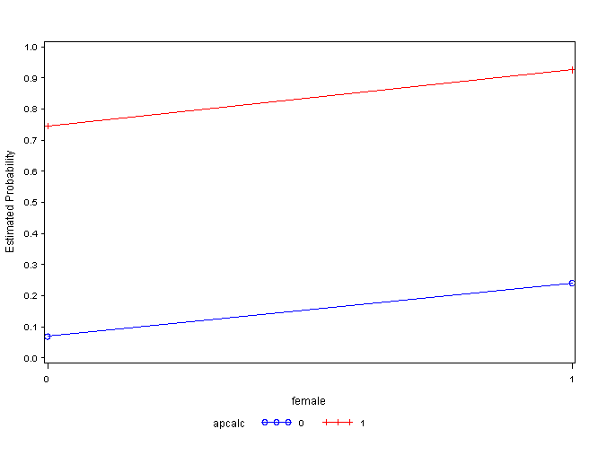
We can also graph the predicted probabilities. To do this, we will
create a new variable called p using the output statement. Then we
will use proc gplot to graph p.
proc logistic data = exlogit desc;
  freq num;
  model admit = female apcalc;
  exact female apcalc / estimate = both;
  output out = pred predicted = p;
run;

symbol1 c=blue v=circle i=join;
symbol2 c=red  v=plus i=join;
symbol3 c=black v=square i=join;
axis1 label=(r=0 a=90) minor=none;
axis2 minor=none order=(0 1);
proc gplot data= pred;
  plot p*female=apcalc / vaxis=axis1 haxis=axis2;
run;
quit;
Things to consider
- Exact logistic regression is a very memory intensive procedure, and it
is relatively easy to exceed the memory capacity of a given computer. - Firth logit may be helpful if you have separation in your data.
You can use the firth option on the model statement to run a Firth
logit. This option was added in SAS version 9.2. - Exact logistic regression is an alternative to conditional logistic
regression if you have stratification, since both condition on the number of
positive outcomes within each stratum. The estimates from these two
analyses will be different because conditional logit conditions only on the
intercept term, while exact logistic regression conditions on the sufficient
statistics of the other regression parameters as well as the intercept term.
See also
- SAS documentation for
proc logistic
References
- Collett, D. Modeling Binary Data, Second Edition. Boca
Raton: Chapman and Hall. - Cox, D. R. and Snell, E. J. (1989). Analysis of Binary Data, Second
Edition. Boca Raton: Chapman and Hall. - Hirji, K. F. (2005). Exact Analysis of Discrete Data. Boca Raton: Chapman
and Hall.