
Version info: Code for this page was tested in SAS 9.3.
Truncated regression is used to model dependent variables for which some of the
observations are not included in the analysis because of the value of the
dependent variable.
Please note: The purpose of this page is to show how to use various data
analysis commands. It does not cover all aspects of the research process which
researchers are expected to do. In particular, it does not cover data
cleaning and checking, verification of assumptions, model diagnostics or
potential follow-up analyses.
Examples of truncated regression
Example 1.
A study of students in a special GATE (gifted and talented education) program
wishes to model achievement as a function of language skills and the type of
program in which the student is currently enrolled. A major concern is
that students are required to have a minimum achievement score of 40 to enter
the special program. Thus, the sample is truncated at an achievement score
of 40.
Example 2. A researcher has data for a sample of Americans whose income is
above the poverty line. Hence, the lower part of the distribution of
income is truncated. If the researcher had a sample of Americans whose
income was at or below the poverty line, then the upper part of the income
distribution would be truncated. In other words, truncation is a result of
sampling only part of the distribution of the outcome variable.
Description of the Data
Let’s pursue Example 1 from above. We have a hypothetical data file,truncreg, with 178 observations. We have a hypothetical data file, https://stats.idre.ucla.edu/wp-content/uploads/2016/02/truncreg.sas7bdat, with 178 observations. The
outcome variable is called achiv, and the language test score
variable is called langscore. The variable prog is a categorical predictor variable with
three levels indicating the type of program in which the students were
enrolled.
Let’s look at the data. It is always a good idea to start with descriptive
statistics.
proc means data = mylib.truncreg;
var achiv langscore;
run;
The MEANS Procedure
Variable Label N Mean Std Dev Minimum Maximum
-------------------------------------------------------------------------------------------------
achiv 178 54.2359551 8.9632299 41.0000000 76.0000000
langscore writing score 178 54.0112360 8.9448964 31.0000000 67.0000000
-------------------------------------------------------------------------------------------------
proc sort data = mylib.truncreg;
by prog;
run;
proc means data = mylib.truncreg;
by prog;
var achiv langscore;
run;
--------------------------------------- type of program=1 ----------------------------------------
The MEANS Procedure
Variable Label N Mean Std Dev Minimum Maximum
-------------------------------------------------------------------------------------------------
achiv 40 51.5750000 7.9707398 42.0000000 68.0000000
langscore writing score 40 51.6750000 9.4391099 31.0000000 67.0000000
-------------------------------------------------------------------------------------------------
--------------------------------------- type of program=2 ----------------------------------------
Variable Label N Mean Std Dev Minimum Maximum
-------------------------------------------------------------------------------------------------
achiv 101 56.8910891 9.0187593 41.0000000 76.0000000
langscore writing score 101 56.7326733 7.5748150 37.0000000 67.0000000
-------------------------------------------------------------------------------------------------
--------------------------------------- type of program=3 ----------------------------------------
Variable Label N Mean Std Dev Minimum Maximum
-------------------------------------------------------------------------------------------------
achiv 37 49.8648649 7.2769124 41.0000000 68.0000000
langscore writing score 37 49.1081081 9.2699748 31.0000000 67.0000000
-------------------------------------------------------------------------------------------------
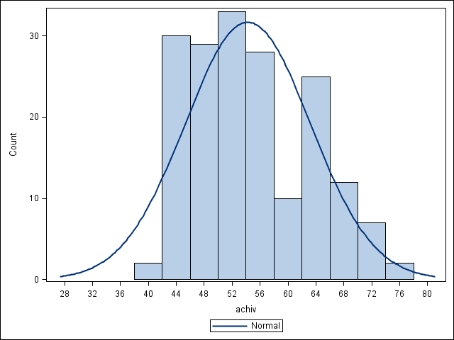
proc sgplot data = mylib.truncreg;
histogram achiv / scale = count showbins;
density achiv;
run;
 proc freq data = mylib.truncreg;
tables prog;
run;
The FREQ Procedure
type of program
Cumulative Cumulative
prog Frequency Percent Frequency Percent
---------------------------------------------------------
1 40 22.47 40 22.47
2 101 56.74 141 79.21
3 37 20.79 178 100.00
proc freq data = mylib.truncreg;
tables prog;
run;
The FREQ Procedure
type of program
Cumulative Cumulative
prog Frequency Percent Frequency Percent
---------------------------------------------------------
1 40 22.47 40 22.47
2 101 56.74 141 79.21
3 37 20.79 178 100.00
Analysis methods you might consider
Below is a list of some analysis methods you may have
encountered. Some of the methods listed are quite reasonable, while others have
either fallen out of favor or have limitations.
- OLS regression – You could analyze these data using OLS regression.
OLS regression will not adjust the estimates of the coefficients to take
into account the effect of truncating the sample at 40, and the coefficients
may be severely biased. This can be conceptualized as a model
specification error (Heckman, 1979). - Truncated regression – Truncated regression addresses the bias
introduced when using OLS regression with truncated data. Note that with truncated regression, the
variance of the outcome variable is reduced compared to the distribution
that is not truncated. Also, if the lower part of the distribution is
truncated, then the mean of the truncated variable will be greater than the
mean from the untruncated variable; if the truncation is from above, the
mean of the truncated variable will be less than the untruncated variable. - These types of models can also be conceptualized as Heckman
selection models, which are used to correct for sampling selection bias.. - Censored regression – Sometimes the concepts of truncation and censoring
are confused. With censored data we have all of the observations, but we don’t know the “true” values of
some of them. With truncation, some of the observations are not included in the analysis
because of the value of the outcome variable. It would be inappropriate to analyze
the data in our example using a censored regression model.
Truncated regression analysis
We will use proc qlim to run our truncated regression analysis. The variables langscore,
prog are predictors in the model, while achiv is the outcome. We will specify that prog is a categorical variable using a class
statement. The lb= option on the endogenous statement indicates the value at which the left truncation
takes place. There is also a ub= option to indicate the value of the right truncation, which
was not needed in this example. We will use the test statement to
obtain the two degree-of-freedom test of prog. To save our
parameter estimates in a dataset we can use later, we specify a dataset name
using the outest option on the proc qlim statement.
proc qlim data = mylib.truncreg outest = mylib.truncreg_outest;
  class prog;
  model achiv = langscore prog;
  endogenous achiv ~ truncated (lb = 40);
  overall_prog: test prog_academic, prog_general = 0;
run;
                                        The QLIM Procedure

                            Summary Statistics of Continuous Responses

                                                                                    N Obs    N Obs
                            Standard                           Lower       Upper    Lower    Upper
Variable        Mean           Error          Type             Bound       Bound    Bound    Bound

 achiv      54.23596        8.963230       Truncated              40


                                     Class Level Information

                                  Class       Levels    Values
                                  prog             3    academic general vocation


                                        Model Fit Summary

                          Number of Endogenous Variables               1
                          Endogenous Variable                      achiv
                          Number of Observations                     178
                          Log Likelihood                      -591.30981
                          Maximum Absolute Gradient           4.46555E-8
                          Number of Iterations                        21
                          Optimization Method               Quasi-Newton
                          AIC                                       1193
                          Schwarz Criterion                         1209

Algorithm converged.


                                        Standard         Approx
Parameter          DF     Estimate      Error    t Value Pr > |t|

Intercept           1    10.165659     6.676185    1.52  0.1278
langscore           1     0.712578     0.114485    6.22  <.0001
prog      academic  1     5.201081     2.306222    2.26  0.0241
prog      general   1     1.135863     2.669958    0.43  0.6705
prog      vocation  0            0            .     .     .
_Sigma              1     8.755314     0.666880   13.13  <.0001
                       Test Results

Test            Type            Statistic    Pr > ChiSq

OVERALL_PROG    Wald                 7.19        0.0274
- The output begins
with summary statistics of the continuous outcome variable. The summary
includes the mean of the outcome variable achiev, as well as the
standard error of the mean. It also indicates that achiev is
truncated at the value of 40. - The Model Fit Summary table gives information about the model, including
the log likelihood and the AIC. These values can be used to compare
models. - In the table called Parameter Estimates, we have the truncated regression coefficients, the standard
error of the coefficients, the t-values, and the p-value associated with each
t-value. - The ancillary statistic _Sigma is equivalent to the standard error of estimate
in OLS regression. The value of 8.76 can be compared to the standard deviation of achievement, which was
8.96. This shows a modest reduction. The output also contains an estimate of the standard
error of _Sigma as well as a t-value and corresponding p-value. - The
variable langscore is statistically significant. A unit
increase in language score leads to a .71 increase in predicted achievement.
The effect of one of the two levels of prog is also significantly
different from the effect of the reference level, level 3. Compared to level
3 of prog, the
predicted achievement for level 2 of prog increases by about 5.20. To determine if
prog itself
is statistically significant, we can use the test statement to obtain the
two degree-of-freedom test of this variable. In the final table in the
output, we see that the variable prog, taken as a whole, is
statistically significant (chi-square = 7.19, p= 0.0274).
We may be interested in obtaining and comparing expected cell means.
We can use the parameter estimates that we saved as a dataset with the outest
option to get SAS to calculate these expected cell means in a data step.
In this dataset we find that our parameters are named “intercept”, “langscore”,
“prog_academic” and “prog_general”. The first row are the estimates themselves,
while the second row are the standard errors. After computing our predictions, we can compare these expected cell means using test statements.
Let’s compare predicted cell means, varying prog type while holding
langscore is at its mean (52.011236 from the means table above).
data _null_;
  set mylib.truncreg_outest;
  where _TYPE_ = "PARM";
  prog_academic = intercept + 54.011236 * langscore + prog_academic;
  prog_general = intercept + 54.011236 * langscore + prog_general;
  prog_vocation = intercept + 54.011236 * langscore;
  file print;
  put "predicted achiv for langscore = mean and prog = academic: " prog_academic;
  put "predicted achiv for langscore = mean and prog = general:  " prog_general;
  put "predicted achiv for langscore = mean and prog = vocation :" prog_vocation;
run;

<**SOME OUTPUT OMITTED**>
predicted achiv for langscore = mean and prog = academic: 53.853932015
predicted achiv for langscore = mean and prog = general:  49.788713629
predicted achiv for langscore = mean and prog = vocation: 48.652851051
In the output we see our put statements, where we printed our estimates. Now using test statements within proc qlm,
we assess whether these predicted means are different from one another.
proc qlim data = mylib.truncreg;
  class prog;
  model achiv = langscore prog;
  endogenous achiv ~ truncated (lb = 40);
  prog1_vs_prog2: test intercept + 54.01124 * langscore + prog_1 = intercept + 54.01124 * langscore + prog_2;
  prog1_vs_prog3: test intercept + 54.01124 * langscore + prog_1 = intercept + 54.01124 * langscore;
  prog2_vs_prog2: test intercept + 54.01124 * langscore + prog_2 = intercept + 54.01124 * langscore;
run;
<**SOME OUTPUT OMITTED**>
                                          Test Results


         Test                Type            Statistic    Pr > ChiSq    Label

         PROG_ACADEMIC_VS_   Wald            3.91         0.0479        intercept +
         GENGERAL                                                       54.01124 * langscore
                                                                        + prog_academic  =
                                                                        intercept + 54.01124
                                                                        * langscore + prog_general
         PROG_ACADEMIC_VS_    Wald            5.09         0.0241       intercept +
         PROG_VOCATION                                                  54.01124 * langscore
                                                                        + prog_academic  =
                                                                        intercept + 54.01124
                                                                        * langscore
         PROG_GENERAL_VS_     Wald            0.18        0.6705        intercept +
         PROG_VOCATION                                                  54.01124 * langscore
                                                                        + prog_general  =
                                                                        intercept + 54.01124
                                                                        * langscore
The effect of level “academic” of prog appears to be significantly different from the effects of levels
“general” and “vocation” of
prog, which do not differ.
The qlim procedure produces neither an R2 nor a pseudo-R2. You can compute
a rough estimate of the degree of association by correlating achiv with the predicted
value and squaring the result. Below, we rerun the analysis, this time
including an output statement to obtain the predicted values. Next,
we use proc corr to get the correlation between the outcome variable (achiv)
and the predicted value (called p_achiv by default), and use the ods
output statement to save the correlation matrix to a data set called corr.
Finally, we use a data step to square the correlation (and round it to four
decimal places), and output the answer to the output window.
proc qlim data=mylib.truncreg;
  class prog;
  model achiv = langscore prog;
  endogenous achiv ~ truncated (lb = 40);
  output out = mylib.trunc_temp predicted;
run;

ods output PearsonCorr=mylib.corr;
proc corr data = mylib.trunc_temp nosimple;
  var achiv p_achiv;
run;

data _null_;
  set mylib.corr;
  if variable = "achiv";
  file print;
  a = round((P_achiv)**2, .0001);
  put "The squared multiple correlation between achieve and the predicted value is " a;
run;

The squared multiple correlation between achieve and the predicted value is 0.3052
The calculated value of approximately .31 is rough estimate of the R2 you would find in an OLS
regression. The squared correlation between the observed and predicted
academic aptitude values is about 0.31, indicating that these predictors
accounted for over 30% of the variability in the outcome variable.
Things to consider
- You need to be careful about what value is used as the truncation value, because it effects
the estimation of the coefficients and standard errors. In the example above, if we had used
ll(39) instead of ll(40), the results would have been slightly
different. It does not matter that
there were no values of 40 in our sample.
See also
- SAS online manual
- Annotated output for truncated
regression
References
- Greene, W. H. 2003. Econometric Analysis, Fifth Edition. Upper Saddle River, NJ: Prentice
Hall. - Heckman, J. J. 1979. Sample selection bias as a
specification error. Econometrica, Volume 47, Number 1, pages
153 – 161. - Long, J. S. 1997. Regression Models for Categorical and Limited Dependent Variables.
Thousand Oaks, CA: Sage Publications.