
Version info: Code for this page was tested in SAS 9.3
Zero-truncated poisson regression is used to model count data for which the value zero cannot occur.
Please Note: The purpose of this page is to show how to use various data analysis commands.
It does not cover all aspects of the research process which researchers are expected to do. In
particular, it does not cover data cleaning and verification, verification of assumptions, model
diagnostics and potential follow-up analyses.
Examples of zero-truncated Poisson regression
Example 1.
A study of length of hospital stay, in days, as a function of age, kind of health insurance and whether
or not the patient died while in the hospital.
Length of hospital stay is recorded as a minimum of at least one day.
Example 2.
A study of the number of journal articles published by tenured faculty as a function of
discipline (fine arts, science, social science, humanities, medical,
etc). To get tenure faculty must publish, therefore, there are no tenured faculty with
zero publications.
Example 3.
A study by the county traffic court on the number of tickets received by teenagers
as predicted by school performance, amount of driver training and gender. Only individuals
who have received at least one citation are in the traffic court files.
Description of the data
Let’s pursue Example 1 from above.
We have a hypothetical data file, ztp, with 1,493 observations available: ztp .
The length of hospital stay variable is stay.
The variable age gives the age group from 1 to 9 which will be treated as
interval in this example.
The variables hmo and died are binary indicator variables
for HMO insured patients and patients who died while in the hospital, respectively.
Let’s look at the data.
proc means data=mylib.ztp;
var stay;
run;
The MEANS Procedure
Analysis Variable : stay Length of Stay
N Mean Std Dev Minimum Maximum
--------------------------------------------------------------------
1493 9.7287341 8.1329081 1.0000000 74.0000000
--------------------------------------------------------------------
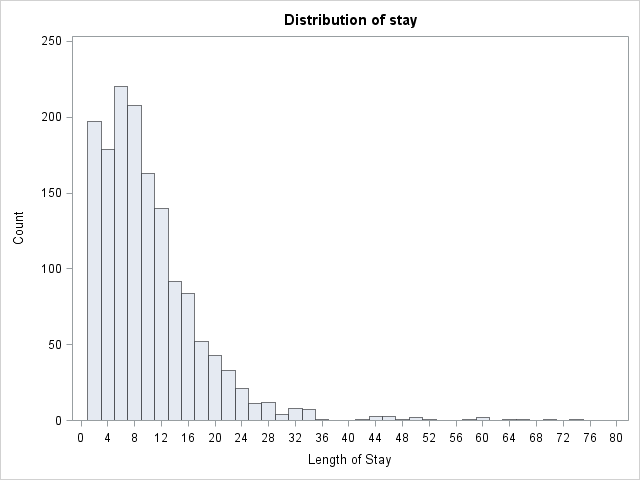
proc univariate data=mylib.ztp noprint;
histogram stay / midpoints = 0 to 80 by 2 vscale = count;
run;
 proc freq data=mylib.ztp;
tables age hmo died;
run;
The FREQ Procedure
Age Group
Cumulative Cumulative
age Frequency Percent Frequency Percent
--------------------------------------------------------
1 6 0.40 6 0.40
2 60 4.02 66 4.42
3 163 10.92 229 15.34
4 291 19.49 520 34.83
5 317 21.23 837 56.06
6 327 21.90 1164 77.96
7 190 12.73 1354 90.69
8 93 6.23 1447 96.92
9 46 3.08 1493 100.00
hmo
Cumulative Cumulative
hmo Frequency Percent Frequency Percent
--------------------------------------------------------
0 1254 83.99 1254 83.99
1 239 16.01 1493 100.00
died
Cumulative Cumulative
died Frequency Percent Frequency Percent
---------------------------------------------------------
0 981 65.71 981 65.71
1 512 34.29 1493 100.00
Analysis methods you might consider
Below is a list of some analysis methods you may have encountered.
Some of the methods listed are quite reasonable while others have either fallen out of favor or
have limitations.
- Zero-truncated Poisson Regression – The focus of this web page.
- Zero-truncated Negative Binomial Regression – If you have overdispersion in addition to
zero truncation. See the Data Analysis Example for
ztnb. - Poisson Regression – Ordinary Poisson regression will have difficulty with
zero-truncated data. It will try to predict zero counts even though there are
no zero values. - Negative Binomial Regression – Ordinary Negative Binomial regression will have difficulty with
zero-truncated data. It will try to predict zero counts even though there are
no zero values. - OLS Regression – You could try to analyze these data using OLS regression. However, count
data are highly non-normal and are not well estimated by OLS regression.
Zero-truncated Poisson regression using proc nlmixed
In order to use proc nlmixed to perform truncated Poisson regression, we must supply it with a likelihood function.
The probability that an observation has count \(y\) under the Poisson
distribution (without zero truncation) is given by the equation:
$$P(Y=y) = \frac{\lambda^y e^{-\lambda}}{y!}$$
With zero truncation, we calculate the probability that \(Y=y\) conditional on \(Y>0\),
that is, that \(Y\) is observed as 0 values are not observed. Thus:
$$P(Y=y|Y>0) = \frac{P(Y=y)}{P(Y>0)} = \frac{P(Y=y)}{1-P(Y=0)} = \frac{\lambda^y e^{-\lambda}}{y!(1-e^{-\lambda})}$$
The log-likelihood function for the zero-truncated Poisson distribution is then:
$$\mathcal{L}=\sum\limits_{i=1}^n[y_ilog(\lambda) – \lambda – log(1 – e^{-\lambda}) – log(y_i!)]$$
In Poisson regression, we model (log(lambda)), the log of the expected
counts, as a linear combination of a set of predictors:
$$log(\lambda) = \beta_0 + \beta_1 x_1 + \beta_2 x_2 + \beta_3 x_3$$
We supply the last two equations to
proc nlmixed to model our data using a zero truncated Poisson distribution.
Additionally, proc nlmixed does not support a class statement, so
categorical variables should be dummy-coded before running the analysis.
proc nlmixed data = mylib.ztp;
	log_lambda = intercept + b_age*age + b_died*died + b_hmo*hmo;
	lambda = exp(log_lambda);
	ll = stay*log_lambda - lambda - log(1-exp(-lambda)) - lgamma(stay+1);
	model stay ~ general(ll);
run;
                                      The NLMIXED Procedure

                                          Specifications

                 Data Set                                    MYLIB.ZTP
                 Dependent Variable                          stay
                 Distribution for Dependent Variable         General
                 Optimization Technique                      Dual Quasi-Newton
                 Integration Method                          None


                                            Dimensions

                             Observations Used                   1493
                             Observations Not Used                  0
                             Total Observations                  1493
                             Parameters                             4


                                            Parameters

                   intercept       b_age      b_died       b_hmo    NegLogLike

                           1           1           1           1    6176595.73


                                         Iteration History

                 Iter     Calls    NegLogLike        Diff     MaxGrad       Slope

                    1         9    21118.0877     6155478    145098.1    -2.38E13
                    2        12    18578.3704    2539.717    137452.3     -436416
                    3        14    18437.2943    141.0761      120107    -13864.4
                    4        16    18394.0864    43.20793    118005.9    -3700.37
                    5        18     17809.511    584.5754    126017.3    -788.358
                    6        20    12597.6045    5211.906     71574.7    -383.804
                    7        21    7312.74337    5284.861    7488.696    -3740.01
                    8        23    7029.45115    283.2922     684.374    -459.944
                    9        25    6943.66162    85.78953    2049.627    -98.7188
                   10        27    6911.69968    31.96194    1391.058    -53.8698
                   11        29    6909.12237    2.577317    98.24019    -4.28966
                   12        31    6908.81335    0.309012    23.25771    -0.33228
                   13        33    6908.80066    0.012691    29.08574    -0.01855
                   14        35    6908.79908    0.001588    0.573832    -0.00203
                   15        37    6908.79907    3.373E-6    0.019132    -6.95E-6


                           NOTE: GCONV convergence criterion satisfied.


                                          The SAS System           09:40 Tuesday, May 29, 2012   2

                                      The NLMIXED Procedure

                                          Fit Statistics

                             -2 Log Likelihood                  13818
                             AIC (smaller is better)            13826
                             AICC (smaller is better)           13826
                             BIC (smaller is better)            13847


                                       Parameter Estimates

                        Standard
   Parameter  Estimate     Error    DF  t Value  Pr > |t|   Alpha     Lower     Upper  Gradient

   intercept    2.4358   0.02733  1493    89.12    <.0001    0.05    2.3822    2.4894  0.003988
   b_age      -0.01444  0.005035  1493    -2.87    0.0042    0.05  -0.02432  -0.00457  0.019132
   b_died      -0.2038   0.01837  1493   -11.09    <.0001    0.05   -0.2398   -0.1677  0.000506
   b_hmo       -0.1359   0.02374  1493    -5.72    <.0001    0.05   -0.1825  -0.08933  -0.00231
The output looks very much like the output from an OLS regression:
- Towards the top is
the iteration history, giving the values of the log pseudolikelihoods. - The last value in the log (-6908.7990731) is the final value
of the log pseudolikelihood for the full model. - Next comes a number of fit statistics, which can be used to compare the fit
of nested models. - Below the fit statistics are the zero-truncated poisson coefficients for each of the variables
along with standard errors, t-scores, and p-values.
Looking through the results we see the following:
- The value of the coefficient for age, -.01444, suggests that the log count of
stay decreases by .01444 for each year increase in age. This coefficient is statistically significant. - The coefficient for hmo, -.1359, is significant and indicates that the log count of stay
for HMO patient is .1359 less than for non-HMO patients. - The log count of stay for patients who died while in the hospital was .20377
less than
those of patients who did not die. - Finally, the value of the constant (intercept), 2..4358 is log count of the stay when
age = 0, hmo = 0, and died = 0.
We can also use estimate statments to help understand our model. For example we can
predict the expected number of days spent at the hospital across age groups for the two hmo statuses
for patients who died. The estimate statement for proc nlmixed works
slightly differently from how it works within other procs. Here, each
parameter must be explicitly multiplied by the value at which is to be held for
that estimate statment. Additionally, because we would like to
predict actual number of days rather than log number of days, we need to
exponentiate the estimate.
proc nlmixed data = mylib.ztp;
	log_lambda = intercept + b_age*age + b_died*died + b_hmo*hmo;
	lambda = exp(log_lambda);
	ll = stay*log_lambda - lambda - log(1-exp(-lambda)) - lgamma(stay+1);
	model stay ~ general(ll);
	estimate 'age 1 died 1 hmo 0' exp(intercept * 1 + b_age * 1 + b_died * 1 + b_hmo * 0);
	estimate 'age 1 died 1 hmo 1' exp(intercept * 1 + b_age * 1 + b_died * 1 + b_hmo * 1);
	estimate 'age 3 died 1 hmo 0' exp(intercept * 1 + b_age * 3 + b_died * 1 + b_hmo * 0);
	estimate 'age 3 died 1 hmo 1' exp(intercept * 1 + b_age * 3 + b_died * 1 + b_hmo * 1);
        estimate 'age 5 died 1 hmo 0' exp(intercept * 1 + b_age * 5 + b_died * 1 + b_hmo * 0);
	estimate 'age 5 died 1 hmo 1' exp(intercept * 1 + b_age * 5 + b_died * 1 + b_hmo * 1);
	estimate 'age 7 died 1 hmo 0' exp(intercept * 1 + b_age * 7 + b_died * 1 + b_hmo * 0);
	estimate 'age 7 died 1 hmo 1' exp(intercept * 1 + b_age * 7 + b_died * 1 + b_hmo * 1);
	estimate 'age 9 died 1 hmo 0' exp(intercept * 1 + b_age * 9 + b_died * 1 + b_hmo * 0);
	estimate 'age 9 died 1 hmo 1' exp(intercept * 1 + b_age * 9 + b_died * 1 + b_hmo * 1);
run;

<**SOME OUTPUT OMITTED**>

                                      Additional Estimates

                                 Standard
   Label               Estimate     Error    DF  t Value  Pr > |t|   Alpha     Lower     Upper

   age 1 died 1 hmo 0    9.1852    0.2548  1493    36.05
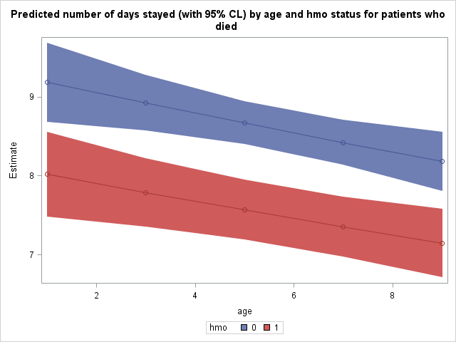
We can see that the number of days spent tends to decrease as we move up age
groups and that patients enrolled in an hmo (hmo = 1) tend to spend fewer days at the hospital as well than those not in hmos. For example, we expect that a non-hmo patient
who died in age group 1 to stay for 9.1852 days whereas an hmo patient who died in age group 1 is expected to stay 8.0180 days.
It may be illustrative for us to plot the predicted number of days stayed
as a function of age and hmo status. To do this, we must tell SAS to save
this table of predicted values as a dataset. Tables and graphics produced
by procedures are given names upon creation. We will need the name of this
prediction table to tell SAS to save it. Place ods trace
on and ods trace off statements around the procedure
which produced this table to obtain its name. Output from the ods
trace
statements is located in the log, not the output.
ods trace on;
proc nlmixed data = mylib.ztp;
	log_lambda = intercept + b_age*age + b_died*died + b_hmo*hmo;
	lambda = exp(log_lambda);
	ll = stay*log_lambda - lambda - log(1-exp(-lambda)) - lgamma(stay+1);
	model stay ~ general(ll);
	estimate 'age 1 died 1 hmo 0' exp(intercept * 1 + b_age * 1 + b_died * 1 + b_hmo * 0);
	estimate 'age 1 died 1 hmo 1' exp(intercept * 1 + b_age * 1 + b_died * 1 + b_hmo * 1);
	estimate 'age 3 died 1 hmo 0' exp(intercept * 1 + b_age * 3 + b_died * 1 + b_hmo * 0);
	estimate 'age 3 died 1 hmo 1' exp(intercept * 1 + b_age * 3 + b_died * 1 + b_hmo * 1);
        estimate 'age 5 died 1 hmo 0' exp(intercept * 1 + b_age * 5 + b_died * 1 + b_hmo * 0);
	estimate 'age 5 died 1 hmo 1' exp(intercept * 1 + b_age * 5 + b_died * 1 + b_hmo * 1);
	estimate 'age 7 died 1 hmo 0' exp(intercept * 1 + b_age * 7 + b_died * 1 + b_hmo * 0);
	estimate 'age 7 died 1 hmo 1' exp(intercept * 1 + b_age * 7 + b_died * 1 + b_hmo * 1);
	estimate 'age 9 died 1 hmo 0' exp(intercept * 1 + b_age * 9 + b_died * 1 + b_hmo * 0);
	estimate 'age 9 died 1 hmo 1' exp(intercept * 1 + b_age * 9 + b_died * 1 + b_hmo * 1);
run;
ods trace off;

<***SOME OF THE LOG OMITTED***>

Output Added:
-------------
Name:       AdditionalEstimates
Label:      Additional Estimates
Template:   Stat.NLM.AdditionalEstimates
Path:       Nlmixed.AdditionalEstimates
-------------
NOTE: PROCEDURE NLMIXED used (Total process time):
      real time           0.20 seconds
      cpu time            0.12 seconds


140  ods trace off;
Towards the end of the log we find the name of this table, which as expected by its heading in the output
above, is “AdditionalEstimates”. We can now tell SAS to save this output
table as the dataset “mylib.addest” using an ods output statement.
ods output AdditionalEstimates = mylib.addest;
proc nlmixed data = mylib.ztp;
	log_lambda = intercept + b_age*age + b_died*died + b_hmo*hmo;
	lambda = exp(log_lambda);
	ll = stay*log_lambda - lambda - log(1-exp(-lambda)) - lgamma(stay+1);
	model stay ~ general(ll);
	estimate 'age 1 died 1 hmo 0' exp(intercept * 1 + b_age * 1 + b_died * 1 + b_hmo * 0);
	estimate 'age 1 died 1 hmo 1' exp(intercept * 1 + b_age * 1 + b_died * 1 + b_hmo * 1);
	estimate 'age 3 died 1 hmo 0' exp(intercept * 1 + b_age * 3 + b_died * 1 + b_hmo * 0);
	estimate 'age 3 died 1 hmo 1' exp(intercept * 1 + b_age * 3 + b_died * 1 + b_hmo * 1);
        estimate 'age 5 died 1 hmo 0' exp(intercept * 1 + b_age * 5 + b_died * 1 + b_hmo * 0);
	estimate 'age 5 died 1 hmo 1' exp(intercept * 1 + b_age * 5 + b_died * 1 + b_hmo * 1);
	estimate 'age 7 died 1 hmo 0' exp(intercept * 1 + b_age * 7 + b_died * 1 + b_hmo * 0);
	estimate 'age 7 died 1 hmo 1' exp(intercept * 1 + b_age * 7 + b_died * 1 + b_hmo * 1);
	estimate 'age 9 died 1 hmo 0' exp(intercept * 1 + b_age * 9 + b_died * 1 + b_hmo * 0);
	estimate 'age 9 died 1 hmo 1' exp(intercept * 1 + b_age * 9 + b_died * 1 + b_hmo * 1);
run;
Now we can use this predicted values for plotting. We need to add actual values of
age and hmo to the dataset for plotting as well.
data mylib.addest;
	set mylib.addest;
	input age hmo;
	datalines;
	1 0
	1 1
	3 0
	3 1
	5 0
	5 1
	7 0
	7 1
	9 0
	9 1
	;
run;
Finally, we use proc sgplot to plot our predicted number of days stayed as well as 95% confidence interval bands. The predicted values,
lines connecting them, and confidence interval bands are all specified
separately within the same proc sgplot. The group option will produce
separate points, lines, and bands by the grouping variable.
proc sgplot data = mylib.addest;
	title 'Predicted number of days stayed (with 95% CL) by age and hmo status for patients who died';
	band x = age lower = lower upper = upper / group=hmo;
	scatter x= age y = estimate / group = hmo;
	series x = age y = estimate / group = hmo;
run;
Zero-truncated Poisson regression using proc fmm
As of SAS 9.3, you can use proc fmm to fit zero-truncated Poisson models.
You simply specify “dist = truncpoisson” in the model statement.
Although compared to proc nlmixed, proc fmm provides a much easier
way to specify a zero-truncated poisson regression, it has much more limited
postestimation options. For example, estimate and predict statements
are not available with proc fmm. Additionally, proc
fmm like most other SAS procs, uses the last group within a categorical
variable as the reference group.
proc fmm data = mylib.ztp;
	class hmo died;
	model stay = age hmo died / dist = truncpoisson;
run;

                                        The FMM Procedure

                                        Model Information

                       Data Set             MYLIB.ZTP
                       Response Variable    stay
                       Type of Model        Homogeneous Regression Mixture
                       Distribution         Truncated Poisson
                       Components           1
                       Link Function        Log
                       Estimation Method    Maximum Likelihood


                                     Class Level Information

                                    Class    Levels    Values

                                    hmo           2    0 1
                                    died          2    0 1


                             Number of Observations Read        1493
                             Number of Observations Used        1493


                                    Optimization Information

                         Optimization Technique        Dual Quasi-Newton
                         Parameters in Optimization    4
                         Mean Function Parameters      4
                         Scale Parameters              0
                         Number of Threads             4


                                         Iteration History

                                              Objective                         Max
               Iteration    Evaluations        Function          Change    Gradient

                       0              5     7444.776354       .            4192.321
                       1              4    6918.2708098    526.50554412    359.7548
                       2              4    6913.2026998      5.06811003    327.6266
                       3              4    6913.0538752      0.14882461    320.7117
                       4              4    6910.8911491      2.16272613    145.0423
                       5              3    6908.8042839      2.08686512    9.443069
                       6              3    6908.7990735      0.00521050     0.07041
                       7              3    6908.7990731      0.00000040    0.000569

                          Convergence criterion (GCONV=1E-8) satisfied.

                                          The SAS System          09:48 Thursday, May 24, 2012  14

                                        The FMM Procedure

                                          Fit Statistics

                               -2 Log Likelihood            13817.6
                               AIC  (smaller is better)     13825.6
                               AICC (smaller is better)     13825.6
                               BIC  (smaller is better)     13846.8
                               Pearson Statistic             9968.8


                        Parameter Estimates for 'Truncated Poisson' Model

                                                     Standard
             Effect       hmo    died    Estimate       Error    z Value    Pr > |z|

             Intercept                     2.0961     0.03766      55.65
Things to consider
- Count data often use exposure variable to indicate the number of times the event could have happened. You can incorporate exposure into your model by including a log-linear term for exposure in the log-likehood function specification.
- It is not recommended that zero-truncated poisson models be applied to
small samples. What constitutes a small sample does not seem to be clearly defined
in the literature. - Pseudo-R-squared values differ from OLS R-squareds, please see
FAQ: What are
pseudo R-squareds? for a discussion on this issue.
References
- Cameron, A. Colin and Trivedi, P.K. (2009) Microeconometrics using stata. College Station, TX: Stata
Press. - Long, J. Scott, & Freese, Jeremy (2006). Regression Models for Categorical Dependent Variables
Using Stata (Second Edition). College Station, TX: Stata Press. - Long, J. Scott (1997). Regression Models for Categorical and Limited Dependent Variables.
Thousand Oaks, CA: Sage Publications.