Applied Linear Statistical Models by Neter, Kutner, et. al. Chapter 23: Multifactor Studies

Inputting table 23.4a, p. 943.

data stress;
  input exercise gender fat smoking rep;
  label gender='1=male, 2=female'
        fat='1=low fat, 2=high fat'
	smoking='1=Light, 2=heavy';
cards;
  24.1  1  1  1  1
  29.2  1  1  1  2
  24.6  1  1  1  3
  20.0  2  1  1  1
  21.9  2  1  1  2
  17.6  2  1  1  3
  14.6  1  2  1  1
  15.3  1  2  1  2
  12.3  1  2  1  3
  16.1  2  2  1  1
   9.3  2  2  1  2
  10.8  2  2  1  3
  17.6  1  1  2  1
  18.8  1  1  2  2
  23.2  1  1  2  3
  14.8  2  1  2  1
  10.3  2  1  2  2
  11.3  2  1  2  3
  14.9  1  2  2  1
  20.4  1  2  2  2
  12.8  1  2  2  3
  10.1  2  2  2  1
  14.4  2  2  2  2
   6.1  2  2  2  3
;
run;

Table 23.4b, p. 943. The cell means and the factor means.

Note: It would be possible to obtain all the means by using multiple proc means but the
lsmeans statement in proc glm is actually more flexible and allows you to obtain all the
means in a single statement. The bars is a special notation which indicates that all the interactions
should be included even the three-way interaction.

ods output  GLM.LSMEANS.gender_fat_smoking.LSMeans=temp;
ods listing close;
proc glm data= stress;
  class gender fat smoking;
  model exercise = gender|fat|smoking ;
  lsmeans gender|fat|smoking;
run;
quit;
proc print data=temp;
run;
ods listing;
data temp1;
  set temp;
  if gender=1 then
    if smoking=2  then heavy_m= exerciseLSMean;
	else if smoking=1  then light_m=exerciseLSMean;
  if gender=2 then
    if smoking=2  then heavy_f= exerciseLSMean;
	else if smoking=1 then light_f=exerciseLSMean; 
  if smoking=1 then
    if fat=2 then light_high = exerciseLSMean;
	else if fat=1 then light_low = exerciseLSMean;
  if smoking=2 then
    if fat=1 then heavy_high = exerciseLSMean;
	else if fat=2 then heavy_low = exerciseLSMean;
run;
goptions reset=all;
symbol1 v=dot c=blue h=.8 i=join;
symbol2 v=dot c=red h=.8 i=join;
axis1 order=(0 to 40 by 10) label=(angle=90 'Minutes of Exercise');
legend1 label=none value=(height=1 font=swiss 'Heavy Smoking' 'Light Smoking' ) 
  position=(bottom right inside) mode=share cborder=black;
legend2 label=none value=(height=1 font=swiss 'Low Fat' 'High Fat' ) 
  position=(bottom right inside) mode=share cborder=black;
proc gplot data = temp1;
  plot (heavy_m light_m)*fat/ overlay vaxis=axis1 legend=legend1 ;
run;
filename outfile 'c:sas2htmhttps://stats.idre.ucla.edu/wp-content/uploads/2016/02/alsm23_2.gif';
goptions gsfmode=replace gsfname=outfile device=gif373; 
  plot (heavy_f light_f)*fat /overlay vaxis=axis1 legend=legend1 ;
run;
  plot (light_low light_high)*gender/ overlay vaxis=axis1 legend=legend2 ;
run;
  plot (heavy_high heavy_low)*gender / overlay vaxis=axis1 legend=legend2 ;
run;
quit;
goptions reset=all;

exercise
Obs Effect gender fat smoking LSMean

1 gender_fat_smoking 1 1 1 25.9666667
2 gender_fat_smoking 1 1 2 19.8666667
3 gender_fat_smoking 1 2 1 14.0666667
4 gender_fat_smoking 1 2 2 16.0333333
5 gender_fat_smoking 2 1 1 19.8333333
6 gender_fat_smoking 2 1 2 12.1333333
7 gender_fat_smoking 2 2 1 12.0666667
8 gender_fat_smoking 2 2 2 10.2000000

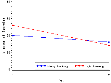
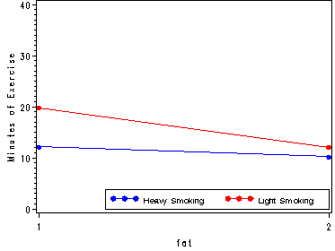
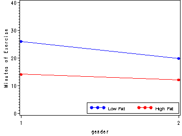
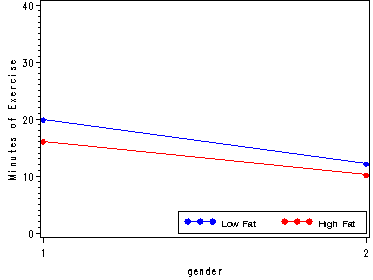
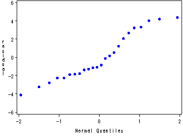
Fig. 23.7 and 23.8, p. 945.

proc glm data=stress;
  class gender fat smoking;
  model exercise = gender|fat|smoking;
  output out=temp r=residual;
run;
quit;
symbol v=dot c=blue h=.8;
proc capability data=temp noprint;
  qqplot residual;
run;

The GLM Procedure

Class Level Information

Class Levels Values
gender 2 1 2
fat 2 1 2
smoking 2 1 2

Number of observations 24

The GLM Procedure

Dependent Variable: exercise
Sum of
Source DF Squares Mean Square F Value Pr > F
Model 7 588.5829167 84.0832738 9.01 0.0002
Error 16 149.3666667 9.3354167
Corrected Total 23 737.9495833

R-Square     Coeff Var      Root MSE    exercise Mean

0.797592      18.77833      3.055391         16.27083

Source DF Type I SS Mean Square F Value Pr > F
gender 1 176.5837500 176.5837500 18.92 0.0005
fat 1 242.5704167 242.5704167 25.98 0.0001
gender*fat 1 13.6504167 13.6504167 1.46 0.2441
smoking 1 70.3837500 70.3837500 7.54 0.0144
gender*smoking 1 11.0704167 11.0704167 1.19 0.2923
fat*smoking 1 72.4537500 72.4537500 7.76 0.0132
gender*fat*smoking 1 1.8704167 1.8704167 0.20 0.6604

Source DF Type III SS Mean Square F Value Pr > F
gender 1 176.5837500 176.5837500 18.92 0.0005
fat 1 242.5704167 242.5704167 25.98 0.0001
gender*fat 1 13.6504167 13.6504167 1.46 0.2441
smoking 1 70.3837500 70.3837500 7.54 0.0144
gender*smoking 1 11.0704167 11.0704167 1.19 0.2923
fat*smoking 1 72.4537500 72.4537500 7.76 0.0132
gender*fat*smoking 1 1.8704167 1.8704167 0.20 0.6604

Estimation of Contrasts of Treatment means, p. 947.
First we obtain the relevant datasets from the output of the proc glm using ods.
Then we create a macro variable for the degrees of freedom that we need in order to obtain the Bonferroni
multiple for a 95% family confidence coefficient. Finally, we get the confidence intervals for each of
the three contrasts, p. 948.

ods output Estimates=temp;
ods output OverallANOVA=anova;
proc glm data=stress;
  class gender fat smoking;
  model exercise = gender|fat|smoking;
  estimate 'L1' smoking 1 -1 fat*smoking 1 -1 0 0;
  estimate 'L2' smoking 1 -1 fat*smoking 0 0 1 -1;
  estimate 'L3' gender 1 -1;
run;
quit;
data _null_;
  set anova;
  if source='Error' then call symput('Df', DF);
run;
%put here is the df we should use &df;
data temp;
 set temp;
 drop dependent tvalue probt;
  B = tinv( 1- (.05/6), &df);
  lower = estimate - B*stderr;
  upper = estimate + B*stderr;
run;
proc print data=temp;
run;

The GLM Procedure

Class Level Information

Class Levels Values
gender 2 1 2
fat 2 1 2
smoking 2 1 2

Number of observations 24

The GLM Procedure

Dependent Variable: exercise
Sum of
Source DF Squares Mean Square F Value Pr > F
Model 7 588.5829167 84.0832738 9.01 0.0002
Error 16 149.3666667 9.3354167
Corrected Total 23 737.9495833

R-Square     Coeff Var      Root MSE    exercise Mean

0.797592      18.77833      3.055391         16.27083

Source                      DF       Type I SS     Mean Square    F Value    Pr > F

gender                       1     176.5837500     176.5837500      18.92    0.0005

fat                          1     242.5704167     242.5704167      25.98    0.0001

gender*fat                   1      13.6504167      13.6504167       1.46    0.2441

smoking                      1      70.3837500      70.3837500       7.54    0.0144

gender*smoking               1      11.0704167      11.0704167       1.19    0.2923

fat*smoking                  1      72.4537500      72.4537500       7.76    0.0132

gender*fat*smoking           1       1.8704167       1.8704167       0.20    0.6604

Source                      DF     Type III SS     Mean Square    F Value    Pr > F

gender                       1     176.5837500     176.5837500      18.92    0.0005

fat                          1     242.5704167     242.5704167      25.98    0.0001

gender*fat                   1      13.6504167      13.6504167       1.46    0.2441

smoking                      1      70.3837500      70.3837500       7.54    0.0144

gender*smoking               1      11.0704167      11.0704167       1.19    0.2923

fat*smoking                  1      72.4537500      72.4537500       7.76    0.0132

gender*fat*smoking           1       1.8704167       1.8704167       0.20    0.6604

                                            Standard

Parameter                   Estimate           Error    t Value    Pr > |t|

L1                        6.90000000      1.76403105       3.91      0.0012

L2                       -0.05000000      1.76403105      -0.03      0.9777

L3                        5.42500000      1.24735832       4.35      0.0005

Obs Parameter Estimate StdErr B lower upper

1 L1 6.90000000 1.76403105 2.67303 2.18469 11.6153
2 L2 -0.05000000 1.76403105 2.67303 -4.76531 4.6653
3 L3 5.42500000 1.24735832 2.67303 2.09077 8.7592

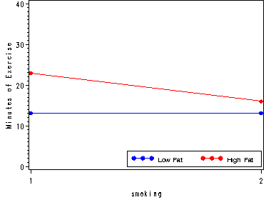
The effects of Body Fat and Smoking History, fig. 23.9b, p. 949.

ods output  GLM.LSMEANS.fat_smoking.LSMeans=temp;
ods listing close;
proc glm data= stress;
  class  fat smoking;
  model exercise = fat smoking fat*smoking ;
  lsmeans fat smoking fat*smoking;
run;
quit;
ods listing;
data temp1;
  set temp;
  if fat=1 then low = exerciseLSMean;
	else if fat=2 then high = exerciseLSMean;
run;
goptions reset=all;
symbol1 v=dot c=blue h=.8 i=join;
symbol2 v=dot c=red h=.8 i=join;
axis1 order=(0 to 40 by 10) label=(angle=90 'Minutes of Exercise');
legend1 label=none value=(height=1 font=swiss 'Low Fat' 'High Fat' ) 
  position=(bottom right inside) mode=share cborder=black;
proc gplot data = temp1;
  plot (high low)*smoking/ overlay vaxis=axis1 legend=legend1 ;
run;
quit;
goptions reset=all;

Creating the Stress data with missing values and generating the indicator variables, table 23.5, p. 950.

data missing;
  set stress;
  if gender=1 and fat=1 and smoking=1 and rep=3 then delete;
  if gender=2 and fat=2 and smoking=1 and rep=2 then delete;
  y = exercise;
  x1 = 1;
  if gender=2 then x1 = -1;
  x2 = 1;
  if fat=2 then x2 = -1;
  x3 = 1;
  if smoking=2 then x3 = -1;
  x12 = x1*x2;
  x13 = x1*x3;
  x23 = x2*x3;
  x123 = x1*x2*x3;
run;
proc print data=missing;
run;

Obs exercise gender fat smoking rep y x1 x2 x3 x12 x13 x23 x123

1 24.1 2 29.2 3 20.0 4 21.9 5 17.6 6 14.6 7 15.3 8 12.3 9 16.1 10 10.8 11 17.6 12 18.8 13 23.2 14 14.8 15 10.3 16 11.3 17 14.9 18 20.4 19 12.8 20 10.1 21 14.4 22 6.1 1 1 1 1 24.1 1 1 1 1 1 1 1
1 1 1 2 29.2 1 1 1 1 1 1 1
2 1 1 1 20.0 -1 1 1 -1 -1 1 -1
2 1 1 2 21.9 -1 1 1 -1 -1 1 -1
2 1 1 3 17.6 -1 1 1 -1 -1 1 -1
1 2 1 1 14.6 1 -1 1 -1 1 -1 -1
1 2 1 2 15.3 1 -1 1 -1 1 -1 -1
1 2 1 3 12.3 1 -1 1 -1 1 -1 -1
2 2 1 1 16.1 -1 -1 1 1 -1 -1 1
2 2 1 3 10.8 -1 -1 1 1 -1 -1 1
1 1 2 1 17.6 1 1 -1 1 -1 -1 -1
1 1 2 2 18.8 1 1 -1 1 -1 -1 -1
1 1 2 3 23.2 1 1 -1 1 -1 -1 -1
2 1 2 1 14.8 -1 1 -1 -1 1 -1 1
2 1 2 2 10.3 -1 1 -1 -1 1 -1 1
2 1 2 3 11.3 -1 1 -1 -1 1 -1 1
1 2 2 1 14.9 1 -1 -1 -1 -1 1 1
1 2 2 2 20.4 1 -1 -1 -1 -1 1 1
1 2 2 3 12.8 1 -1 -1 -1 -1 1 1
2 2 2 1 10.1 -1 -1 -1 1 1 1 -1
2 2 2 2 14.4 -1 -1 -1 1 1 1 -1
2 2 2 3 6.1 -1 -1 -1 1 1 1 -1

Testing factor A (Gender) by dropping x1 from the full model and regressing y on the variables
in column 3-8, p. 950.

proc reg data=missing;
  model y = x1-x3 x12 x13 x23 x123;
  model y = x2 x3 x12 x13 x23 x123;
run;
quit;

The REG Procedure
Model: MODEL1
Dependent Variable: y

Analysis of Variance

Sum of Mean
Source DF Squares Square F Value Pr > F
Model 7 484.81485 69.25926 7.18 0.0009
Error 14 135.08333 9.64881
Corrected Total 21 619.89818

Root MSE 3.10625 R-Square 0.7821
Dependent Mean 16.20909 Adj R-Sq 0.6731
Coeff Var 19.16365

Parameter Estimates

Parameter Standard
Variable DF Estimate Error t Value Pr > |t|
Intercept 1 16.52917 0.67252 24.58 <.0001
x1 1 2.62500 0.67252 3.90 0.0016
x2 1 3.09167 0.67252 4.60 0.0004
x3 1 1.97083 0.67252 2.93 0.0110
x12 1 1.01250 0.67252 1.51 0.1544
x13 1 -0.76667 0.67252 -1.14 0.2734
x23 1 1.65000 0.67252 2.45 0.0279
x123 1 0.53750 0.67252 0.80 0.4375

The REG Procedure
Model: MODEL2
Dependent Variable: y

Analysis of Variance

Sum of Mean
Source DF Squares Square F Value Pr > F
Model 6 337.81485 56.30247 2.99 0.0397
Error 15 282.08333 18.80556
Corrected Total 21 619.89818

Root MSE 4.33654 R-Square 0.5450
Dependent Mean 16.20909 Adj R-Sq 0.3629
Coeff Var 26.75374

Parameter Estimates

Parameter Standard
Variable DF Estimate Error t Value Pr > |t|
Intercept 1 16.52917 0.93889 17.61 <.0001
x2 1 2.80000 0.93307 3.00 0.0090
x3 1 1.97083 0.93889 2.10 0.0531
x12 1 1.01250 0.93889 1.08 0.2979
x13 1 -1.05833 0.93307 -1.13 0.2745
x23 1 1.35833 0.93307 1.46 0.1661
x123 1 0.53750 0.93889 0.57 0.5755