
Inputting the Apex Enterprises data, table 24.1, p. 964.
data ratings;
  input rating officer candidate;
cards;
  76  1  1
  65  1  2
  85  1  3
  74  1  4
  59  2  1
  75  2  2
  81  2  3
  67  2  4
  49  3  1
  63  3  2
  61  3  3
  46  3  4
  74  4  1
  71  4  2
  85  4  3
  89  4  4
  66  5  1
  84  5  2
  80  5  3
  79  5  4
;
run;
Officer factor means and grand mean, table 24.1, p. 964.
Note: The grand mean is the first observation that has a missing value for the level of officer.
proc means data = ratings mean noprint;
  class officer;
  var rating;
  output out=temp mean=mout;
run;
proc print data=temp;
  var officer mout;
run;
Obs officer mout1 . 71.45
2 1 75.00
3 2 70.50
4 3 54.75
5 4 79.75
6 5 77.25
Fig. 24.2, p. 964.
goptions reset=all;
symbol c=blue v=dot h=.8;
axis1 label=(a=90 'Treatment');
proc gplot data=ratings;
  plot officer*rating / vaxis=axis1;
run;
quit;
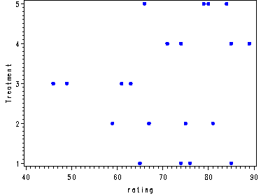
Table 24.2, p. 965.
proc glm data=ratings;
  class officer;
  model rating= officer;
  random officer;
run;
quit;
The GLM ProcedureClass Level Information
Class Levels Values
officer 5 1 2 3 4 5Number of observations 20
The GLM Procedure
Dependent Variable: rating
Sum of
Source DF Squares Mean Square F Value Pr > F
Model 4 1579.700000 394.925000 5.39 0.0068
Error 15 1099.250000 73.283333
Corrected Total 19 2678.950000
R-Square Coeff Var Root MSE rating Mean
0.589671 11.98120 8.560569 71.45000
Source DF Type I SS Mean Square F Value Pr > F
officer 4 1579.700000 394.925000 5.39 0.0068
Source DF Type III SS Mean Square F Value Pr > F
officer 4 1579.700000 394.925000 5.39 0.0068The GLM Procedure
Source Type III Expected Mean Square
officer Var(Error) + 4 Var(officer)
Estimating the overall mean and calculating the 90% confidence limit, p. 967.
Note: There does not appear to be an build in function for this in SAS. So, we will first run
the proc glm again and save the Ybar, the MSTR and the df that we need as macro variables. Then we
calculate the appropriate t-value and finally we compute the confidence limits.
ods listing close;
ods output  OverallANOVA=anova   FitStatistics=fits;
proc glm data=ratings;
  class officer;
  model rating= officer;
  random officer;
run;
quit;
ods listing;
data _null_;
  set anova;
  if source = 'Model' then call symput( 'mstr', ms);
  if source = 'Corrected Total' then call symput('df', df);
run;
%put here are the macro vars: &mstr and &df;
data _null_;
  set fits;
  call symput('mean',  DepMean);
run;
%put here is the last value: &mean;
data temp;
  t = tinv( .95, 4);
  df = &df+1;
  s2 = &mstr/(&df +1);
  Lower = &mean - t*sqrt(s2);
  Upper = &mean + t*sqrt(s2);
run;
proc print data=temp;
run;
Obs t df s2 Lower Upper1 2.13185 20 19.7463 61.9768 80.9232
Estimating the 90% confidence limit of simga_mu2/(sigma_mu2 + sigma2), p. 968-969.
ods listing close;
ods output overallanova=anova;
proc glm data=ratings;
   class officer;
   model rating = officer;
run;
quit;
ods listing;
data _null_;
  set anova;
  if source='Model' then call symput('mstr', ms);
  if source='Error' then call symput('mse', ms);
  if source='Model' then call symput('dfmodel', df);
  if source='Error' then call symput('dferr', df);
run;
%put here are the macro variables:      394.925, &mse, &dfmodel and &dferr;
data temp;
  lower_f = finv( .95, &dfmodel, &dferr);
  upper_f = finv( .05, &dfmodel, &dferr);
  mstr =      394.925;
  mse = &mse;
  L = (1/4)*( (     394.925/&mse)*(1/lower_f) - 1 );
  U = (1/4)*( (     394.925/&mse)*(1/upper_f) - 1 );
  L_star = L/(1+L);
  U_star = U/(1+U);
run;
proc print data=temp;
run;
Obs lower_f upper_f mstr mse L U L_star U_star1 3.05557 0.17071 394.925 73.2833 0.19092 7.64195 0.16031 0.88429
Estimating sigma2 and the 90% confidence interval, p. 970.
Note: We are using the same numbers from the ANOVA table of the proc glm so we will be using the macro
variables that were created when we were estimating the 90% confidence limit of simga_mu2/(sigma_mu2 + sigma2)
on p. 968.
%put here are the macro variables we will be using in this procedure: &mse and &dferr;
data temp;
  mse = &mse;
  dfden = &dferr;
  lower_chi = cinv( .95, &dferr);
  upper_chi = cinv( .05, &dferr);
  lower2 = (&dferr*&mse )/lower_chi;
  upper2 = (&dferr*&mse )/upper_chi;
  lower = sqrt(lower2);
  upper = sqrt(upper2);
run;
proc print data=temp;
run;
lower_ upper_
Obs mse dfden chi chi lower2 upper2 lower upper1 73.2833 15 24.9958 7.26094 43.9774 151.392 6.63155 12.3042
Point estimate and 90% confidence interval for sigma_mu2, p. 972-973.
Note: We are using the same numbers from the ANOVA table of the proc glm so we will be using the macro
variables that were created when we were estimating the 90% confidence limit of simga_mu2/(sigma_mu2 + sigma2)
on p. 968.
%put here are the macro variables that we are using in this calculation: &mstr and &mse;
data temp;
  s_mu2 = ( &mstr - &mse)/4;
  df = round( (4*s_mu2)**2/( (&mstr**2)/(5-1) + (&mse**2)/( 5*(4-1) ) ), 1);
  lower_chi = cinv( .95, df);
  upper_chi = cinv( .05, df);
  lower2 = (df*s_mu2)/lower_chi;
  upper2 = (df*s_mu2)/upper_chi;
  lower = sqrt(lower2);
  upper = sqrt(upper2);
run;
proc print data=temp;
run;
lower_ upper_
Obs s_mu2 df chi chi lower2 upper2 lower upper1 80.4104 3 7.81473 0.35185 30.8688 685.615 5.55597 26.1843
Estimating the 90% confidence interval of s_mu2 using the MLS procedure, p. 974-5.
Note: We are using the same numbers from the ANOVA table of the proc glm so we will be using the
macro variables that were created when we were estimating the 90% confidence limit of simga_mu2/(sigma_mu2 + sigma2)
on p. 968.
Note: When calculating the value of the F distribution SAS won’t allow you to use infinity but
instead we use 1000000000 as an approximation of infinity.
data temp;
  c1 = 1/4;
  c2 = -1/4;
  ms1 = &mstr;
  ms2 = &mse;
  df1= &dfmodel;
  df2= &dferr;
  L = ( &mstr - &mse)/4;
  f1 = finv(.95, df1, 1000000000 );
  f2 = finv(.95, df2, 1000000000);
  f3 = finv(.95, 1000000000, df1);
  f4 = finv(.95, 1000000000, df2);
  f5 = finv(.95, df1, df2);
  f6 = finv(.95, df2, df1);
  g1 = 1 - 1/f1;
  g2 = 1 - 1/f2;
  g3 = ( (f5 - 1)**2 - (g1*f5)**2 - (f4-1)**2 )/f5;
  g4 = f6*( ( (f6-1)/f6 )**2 - ( (f3-1)/f6 )**2 - g2**2 );
  H_lower = sqrt( (g1*c1*ms1)**2 + ( (f4-1)*c2*ms2 )**2 - g3*c1*c2*ms1*ms2 ) ;
  H_upper = sqrt( ( (f3-1)*c1*ms1 )**2 + (g2*c2*ms2)**2 - g4*c1*c2*ms1*ms2 ) ;
  lower2 = L - H_lower;
  upper2 = L + H_upper;
  lower = sqrt(lower2);
  upper = sqrt(upper2);
run;
proc print data=temp;
run;
Obs c1 c2 ms1 ms2 df1 df2 L f1 f2 f3 f4 f5 f61 0.25 -0.25 394.925 73.2833 4 15 80.4104 2.37193 1.66639 5.62807 2.06585 3.05557 5.85781
Obs g1 g2 g3 g4 H_lower H_upper lower2 upper2 lower upper
1 0.57840 0.39990 -0.011190 -0.56475 60.1848 455.875 20.2256 536.285 4.49729 23.1578
The training example p. 982-983, 987-988 and 989 was omitted because the data is not available.
Inputting Sheffield Foods Co. data, table 24.11, p. 995.
data Sheffield;
  input fat method lab rep ;
cards;
5.19  1  1  1
5.09  1  1  2
4.09  1  2  1
3.99  1  2  2
3.75  1  2  3
4.04  1  2  4
4.06  1  2  5
4.62  1  3  1
4.32  1  3  2
4.35  1  3  3
4.59  1  3  4
3.71  1  4  1
3.86  1  4  2
3.79  1  4  3
3.63  1  4  4
3.26  2  1  1
3.48  2  1  2
3.24  2  1  3
3.41  2  1  4
3.35  2  1  5
3.04  2  1  6
3.02  2  2  1
3.32  2  2  2
2.83  2  2  3
2.96  2  2  4
3.23  2  2  5
3.07  2  2  6
3.08  2  3  1
2.95  2  3  2
2.98  2  3  3
2.74  2  3  4
3.07  2  3  5
2.70  2  3  6
2.98  2  4  1
2.89  2  4  2
2.75  2  4  3
3.04  2  4  4
2.88  2  4  5
3.20  2  4  6
;
run;
Fig. 24.3, p. 995.
goptions reset=all;
symbol v=dot h=.8 c=blue;
axis1 order=(0 to 5 by 1) label=(a=90 'Laboratory');
axis2 order=(2.5 to 5.5 by 1);
proc gplot data=sheffield;
  by method;
  plot lab*fat/ vaxis=axis1 haxis=axis2;
run;
quit;
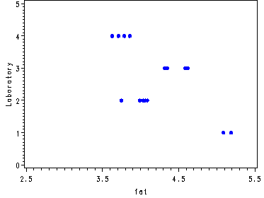
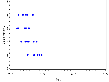
Fig. 24.4, p. 996.
Note: First we need to calculate the means using proc sql and then we create the graph.
proc sql;
  create table plot as
  select method, lab, mean(fat) as mfat
  from sheffield
  where method=1
  group by lab;
quit;
proc sql;
  create table plot1 as
  select method, lab, mean(fat) as mfat1
  from sheffield
  where method=2
  group by lab;
quit;
data combo;
  set plot plot1;
run;
symbol1 c=blue v=dot h=.8 i=join;
symbol2 c=red v=square h=.8 i=join;
axis1 label=(a=90 'Mean');
legend1 label=none value=(height=1 font=swiss 'Method 1' 'Method 2' )
        position=(bottom right inside) mode=share cborder=black;
proc gplot data=combo;
  plot (mfat mfat1)*lab / vaxis=axis1 overlay legend=legend1;
run;
quit;
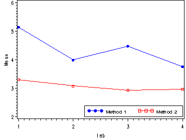
Table 24.13-24.14 and fig. 24.5 were not generated, p. 1000-1001.