
Inputting the Cracker Promotion data, p. 1020.
data cracker;
   input y x treat store;
cards;
  38  21  1  1
  39  26  1  2
  36  22  1  3
  45  28  1  4
  33  19  1  5
  43  34  2  1
  38  26  2  2
  38  29  2  3
  27  18  2  4
  34  25  2  5
  24  23  3  1
  32  29  3  2
  31  30  3  3
  21  16  3  4
  28  29  3  5
;
run;
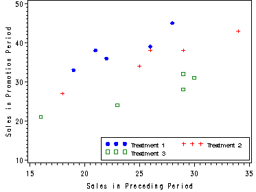
Fig. 25.5, p. 1021.
Note: In order to graph all three treatments at once we need to create three variables where each is equal to
y if treat is equal to a specific treatment but missing otherwise.
data cplot;
  set cracker;
  if treat=1 then treat1 = y;
  else if treat=2 then treat2=y;
  else treat3=y;
run;
goptions reset=all;
symbol1 c=blue v=dot h=.8;
symbol2 c=red v=dot h=.8;
symbol3 c=green v=dot h=.8;
axis1 order=(10 to 50 by 10) label=(a=90 'Sales in Promotion Period');
axis2 order=(15 to 35 by 5) label=('Sales in Preceding Period');
legend1 label=none value=(height=1 font=swiss 'Treatment 1' 'Treatment 2' 'Treatment 3' )
        position=(bottom right inside) mode=share cborder=black;
proc gplot data=cplot;
  plot (treat1 treat2 treat3)*x/overlay legend=legend1 vaxis=axis1 haxis=axis2;
run;
quit;
Creating the indicator and interaction variables for the Cracker data set. First we need to calculate
the overall mean which will be used to generate the x variable (x = X-mean), table 25.2, p. 1021.
proc sql;
  create table cdummy as
  select *, x-mean(x) as littlex
  from cracker;
quit;
data cdummy;
   set cdummy;
   I1 = 0;
   if treat=1 then I1=1;
     else if treat=3 then I1=-1;
   I2=0;
   if treat=2 then I2=1;
     else if treat=3 then I2=-1;
   I1x = I1*littlex;
   I2x = I2*littlex;
run;
proc print data=cdummy;
run;
Obs y x treat store littlex I1 I2 I1x I2x1 38 21 1 1 -4 1 0 -4 0
2 39 26 1 2 1 1 0 1 0
3 36 22 1 3 -3 1 0 -3 0
4 45 28 1 4 3 1 0 3 0
5 33 19 1 5 -6 1 0 -6 0
6 43 34 2 1 9 0 1 0 9
7 38 26 2 2 1 0 1 0 1
8 38 29 2 3 4 0 1 0 4
9 27 18 2 4 -7 0 1 0 -7
10 34 25 2 5 0 0 1 0 0
11 24 23 3 1 -2 -1 -1 2 2
12 32 29 3 2 4 -1 -1 -4 -4
13 31 30 3 3 5 -1 -1 -5 -5
14 21 16 3 4 -9 -1 -1 9 9
15 28 29 3 5 4 -1 -1 -4 -4
Regressing Y on littlex, I1 and I2, table 25.3, p. 1022. Testing for treatment effect, p. 1023-1024.
proc reg data=cdummy outest=outregc covout;
  model y = littlex I1 I2;
  treatment_effect: test I1=I2=0;
  output out=residualc r=resid;
run;
quit;
proc print data=outregc;
  where _type_ = 'COV';
  var intercept littlex I1 I2;
run;
The REG Procedure
Model: MODEL1
Dependent Variable: yAnalysis of Variance
Sum of Mean
Source DF Squares Square F Value Pr > F
Model 3 607.82869 202.60956 57.78 <.0001
Error 11 38.57131 3.50648
Corrected Total 14 646.40000Root MSE 1.87256 R-Square 0.9403
Dependent Mean 33.80000 Adj R-Sq 0.9241
Coeff Var 5.54012Parameter Estimates
Parameter Standard
Variable DF Estimate Error t Value Pr > |t|
Intercept 1 33.80000 0.48349 69.91 <.0001
littlex 1 0.89856 0.10258 8.76 <.0001
I1 1 6.01741 0.70826 8.50 <.0001
I2 1 0.94202 0.69868 1.35 0.2047The REG Procedure
Model: MODEL1Test treatment_effect Results for Dependent Variable y
Mean
Source DF Square F Value Pr > F
Numerator 2 208.57546 59.48 <.0001
Denominator 11 3.50648
Obs Intercept littlex I1 I22 0.23377 0.000000 0.00000 0.00000
3 0.00000 0.010524 0.01894 -0.01473
4 0.00000 0.018943 0.50163 -0.26029
5 0.00000 -0.014733 -0.26029 0.48816
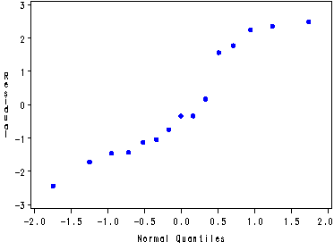
Fig. 25.6b, p. 1023.
goptions reset=all;
symbol c=blue v=dot h=.8;
proc capability data=residualc noprint;
  qqplot resid;
run;
Reduced model–without I1 and I2, table 25.4, p. 1023.
proc reg data=cdummy ;
  model y = littlex ;
run;
quit;
The REG Procedure
Model: MODEL1
Dependent Variable: yAnalysis of Variance
Sum of Mean
Source DF Squares Square F Value Pr > F
Model 1 190.67778 190.67778 5.44 0.0364
Error 13 455.72222 35.05556
Corrected Total 14 646.40000Root MSE 5.92077 R-Square 0.2950
Dependent Mean 33.80000 Adj R-Sq 0.2408
Coeff Var 17.51708
Parameter EstimatesParameter Standard
Variable DF Estimate Error t Value Pr > |t|
Intercept 1 33.80000 1.52874 22.11 <.0001
littlex 1 0.72778 0.31205 2.33 0.0364
Estimation of treatment effects, pair-wise comparisons using proc glm, p. 1024.
ods output Estimates=temp  OverallANOVA=anova;
proc glm data=cracker;
  class treat;
  model y = x treat;
  estimate 'treat1 v treat2' treat 1 -1 0;
  estimate 'treat1 v treat3' treat 1 0 -1;
  estimate 'treat2 v treat3' treat 0 1 -1;
run;
quit;
data _null_;
  set anova;
  if source='Model' then call symput('dfmodel', DF);
  if source='Error' then call symput('dferr', DF);
run;
%put check macro variables in log: &dfmodel and &dferr;
data temp;
  set temp;
  drop dependent tvalue probt;
  S2 =  (&dfmodel - 1)*finv(.95, (&dfmodel - 1), &dferr);
  S = sqrt(S2);
  lower = estimate - S*stderr;
  upper = estimate + S*stderr;
run;
proc print data=temp;
run;
The GLM ProcedureClass Level Information
Class Levels Values
treat 3 1 2 3Number of observations 15
The GLM Procedure
Dependent Variable: ySum of
Source DF Squares Mean Square F Value Pr > F
Model 3 607.8286915 202.6095638 57.78 <.0001
Error 11 38.5713085 3.5064826
Corrected Total 14 646.4000000R-Square Coeff Var Root MSE y Mean
0.940329 5.540120 1.872560 33.80000Source DF Type I SS Mean Square F Value Pr > F
x 1 190.6777778 190.6777778 54.38 <.0001
treat 2 417.1509137 208.5754568 59.48 <.0001
Source DF Type III SS Mean Square F Value Pr > F
x 1 269.0286915 269.0286915 76.72 <.0001
treat 2 417.1509137 208.5754568 59.48 <.0001Standard
Parameter Estimate Error t Value Pr > |t|
treat1 v treat2 5.0753902 1.22896513 4.13 0.0017
treat1 v treat3 12.9768307 1.20562330 10.76 <.0001
treat2 v treat3 7.9014406 1.18874585 6.65 <.0001Obs Parameter Estimate StdErr S2 S lower upper
1 treat1 v treat2 5.0753902 1.22896513 7.96460 2.82216 1.60705 8.5437
2 treat1 v treat3 12.9768307 1.20562330 7.96460 2.82216 9.57437 16.3793
3 treat2 v treat3 7.9014406 1.18874585 7.96460 2.82216 4.54661 11.2563
Estimating the mean response for each treatment group when X is at its mean (X=25), p. 1026.
Note: The output in SAS includes the estimate and the standard error of the estimate which is the square root
of the variance.
proc means data=cracker mean;
  var x;
run;
proc glm data=cracker;
  class treat;
  model y = x treat;
  estimate 'treat1 at X=25' intercept 1 treat 1 0 0 x 25;
  estimate 'treat2 at X=25' intercept 1 treat 0 1 0 x 25;
  estimate 'treat3 at X=25' intercept 1 treat 0 0 1 x 25;
run;
quit;
The MEANS Procedure
Analysis Variable : xMean
————
25.0000000
————The GLM Procedure
Class Level Information
Class Levels Values
treat 3 1 2 3Number of observations 15
The GLM Procedure
Dependent Variable: y
Sum of
Source DF Squares Mean Square F Value Pr > F
Model 3 607.8286915 202.6095638 57.78 <.0001
Error 11 38.5713085 3.5064826
Corrected Total 14 646.4000000R-Square Coeff Var Root MSE y Mean
0.940329 5.540120 1.872560 33.80000Source DF Type I SS Mean Square F Value Pr > F
x 1 190.6777778 190.6777778 54.38 <.0001
treat 2 417.1509137 208.5754568 59.48 <.0001
Source DF Type III SS Mean Square F Value Pr > F
x 1 269.0286915 269.0286915 76.72 <.0001
treat 2 417.1509137 208.5754568 59.48 <.0001Standard
Parameter Estimate Error t Value Pr > |t|
treat1 at X=25 39.8174070 0.85755068 46.43 <.0001
treat2 at X=25 34.7420168 0.84966045 40.89 <.0001
treat3 at X=25 26.8405762 0.83843921 32.01 <.0001
Table 25.5 and testing for parallel slopes, in other words, testing to see if the interactions are
significant, p. 1027.
proc reg data=cdummy;
  model y = littlex I1 I2 I1x I2x;
  interaction: test I1x=I2x=0;
run;
quit;
The REG Procedure
Model: MODEL1
Dependent Variable: yAnalysis of Variance
Sum of Mean
Source DF Squares Square F Value Pr > F
Model 5 614.87916 122.97583 35.11 <.0001
Error 9 31.52084 3.50232
Corrected Total 14 646.40000Root MSE 1.87145 R-Square 0.9512
Dependent Mean 33.80000 Adj R-Sq 0.9241
Coeff Var 5.53683Parameter Estimates
Parameter Standard
Variable DF Estimate Error t Value Pr > |t|
Intercept 1 33.89433 0.51234 66.16 <.0001
littlex 1 0.93874 0.11267 8.33 <.0001
I1 1 6.26990 0.75167 8.34 <.0001
I2 1 0.71791 0.71600 1.00 0.3422
I1x 1 0.15251 0.18438 0.83 0.4296
I2x 1 0.05252 0.14561 0.36 0.7267The REG Procedure
Model: MODEL1Test interaction Results for Dependent Variable y
Mean
Source DF Square F Value Pr > F
Numerator 2 3.52524 1.01 0.4032
Denominator 9 3.50232
Inputting the Salable Flowers data set, table 25.6, p. 1029.
data flowers;
  input y x a b rep;
  label y = 'yield'
        x = 'plot size'
	a = 'variety'
	b = 'moisture';
cards;
  98  15  1  1  1
  60   4  1  1  2
  77   7  1  1  3
  80   9  1  1  4
  95  14  1  1  5
  64   5  1  1  6
  55   4  2  1  1
  60   5  2  1  2
  75   8  2  1  3
  65   7  2  1  4
  87  13  2  1  5
  78  11  2  1  6
  71  10  1  2  1
  80  12  1  2  2
  86  14  1  2  3
  82  13  1  2  4
  46   2  1  2  5
  55   3  1  2  6
  76  11  2  2  1
  68  10  2  2  2
  43   2  2  2  3
  47   3  2  2  4
  62   7  2  2  5
  70   9  2  2  6
;
run;
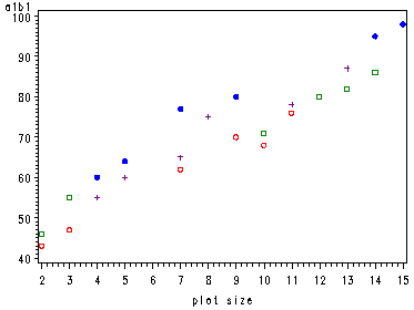
Fig. 25.7, p. 1030.
data fplot;
  set flowers;
  if a=1 and b=1 then a1b1 = y;
  if a=1 and b=2 then a1b2 = y;
  if a=2 and b=1 then a2b1 = y;
  if a=2 and b=2 then a2b2 = y;
run;

symbol1 v=dot c=blue h=.8;
symbol2 v=circle c=red h=.8;
symbol3 v=square c=green h=.8;
symbol4 v=plus c=purple h=.8;
proc gplot data=fplot;
  plot (a1b1 a2b2 a1b2 a2b1)*x/overlay;
run;
quit;
Generating the variable for X centered at its mean, the indicator variables and their
interactions, p. 1028.
proc sql;
  create table fdummy as
  select *, x - mean(x) as littlex
  from  flowers;
quit;
data fdummy;
  set fdummy;
  I1 = 1;
  if a=2 then I1=-1;
  I2 = 1;
  if b=2 then I2=-1;
  I12 = I1*I2;
run;
Table 25.7, regression output and sums of squares, p. 1030 and the test of the interaction, p. 1031.
proc reg data=fdummy;
  model y = littlex I1 I2 I12/ ss2;
  interaction: test I12=0;
run;
quit;
The REG Procedure
Model: MODEL1
Dependent Variable: y yieldAnalysis of Variance
Sum of Mean
Source DF Squares Square F Value Pr > F
Model 4 4966.51882 1241.62970 197.45 <.0001
Error 19 119.48118 6.28848
Corrected Total 23 5086.00000Root MSE 2.50768 R-Square 0.9765
Dependent Mean 70.00000 Adj R-Sq 0.9716
Coeff Var 3.58241Parameter Estimates
Parameter Standard
Variable Label DF Estimate Error t Value Pr > |t| Type II SS
Intercept Intercept 1 70.00000 0.51188 136.75 <.0001 117600
littlex 1 3.27688 0.13002 25.20 <.0001 3994.51882
I1 1 2.04234 0.52108 3.92 0.0009 96.60183
I2 1 3.68078 0.51291 7.18 <.0001 323.84947
I12 1 0.81922 0.51291 1.60 0.1267 16.04224The REG Procedure
Model: MODEL1Test interaction Results for Dependent Variable y
Mean
Source DF Square F Value Pr > F
Numerator 1 16.04224 2.55 0.1267
Denominator 19 6.28848
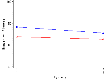
Fig. 25.8, estimated treatment means plot (x=0).
ods listing close;
ods output  LSMeans=means;
proc glm data=flowers;
  class a b;
  model y = x a b a*b;
  estimate 'Factor A effect' a 1 -1;
  estimate 'Factor B effect' b 1 -1;
  lsmeans a*b;
run;
quit;
ods output close;
ods listing;
data means;
  set means;
  a1=a+0;
  if b=1 then b1=yLSMean;
  if b=2 then b2=yLSMean;
run;
filename outfile 'c:sas2htmhttps://stats.idre.ucla.edu/wp-content/uploads/2016/02/alsm25_4.gif';
goptions gsfname=outfile dev=gif373;
symbol1 v=dot c=blue i=join;
symbol2 v=circle c=red i=join;
axis1 offset = (2, 2) label=('Variety') ;
axis2 order=(40 to 100 by 20) label=(a=90 'Number of Flowers');
proc gplot data=means;
  plot (b1 b2)*a / overlay haxis=axis1 vaxis=axis2;
run;
quit;
Testing the Factor effects using proc glm, p. 1031-1032.
ods output Estimates=temp  OverallANOVA=anova;
proc glm data=flowers;
  class a b;
  model y = x a b a*b;
  estimate 'Factor A effect' a 1 -1;
  estimate 'Factor B effect' b 1 -1;
run;
quit;
data _null_;
  set anova;
  if source='Error' then call symput('dferr', DF);
run;
%put check macro variables in log: &dferr;
data temp;
  set temp;
  drop dependent tvalue probt;
  t = tinv( (1 - .05/(2*2) ), &dferr);
  lower = estimate - t*stderr;
  upper = estimate + t*stderr;
run;
proc print data=temp;
run;
The GLM ProcedureClass Level Information
Class Levels Values
a 2 1 2
b 2 1 2Number of observations 24
The GLM Procedure
Dependent Variable: y yield
Sum of
Source DF Squares Mean Square F Value Pr > F
Model 4 4966.518817 1241.629704 197.45 <.0001
Error 19 119.481183 6.288483
Corrected Total 23 5086.000000R-Square Coeff Var Root MSE y Mean
0.976508 3.582407 2.507685 70.00000Source DF Type I SS Mean Square F Value Pr > F
x 1 4532.635779 4532.635779 720.78 <.0001
a 1 93.406888 93.406888 14.85 0.0011
b 1 324.433906 324.433906 51.59 <.0001
a*b 1 16.042244 16.042244 2.55 0.1267Source DF Type III SS Mean Square F Value Pr > F
x 1 3994.518817 3994.518817 635.21 <.0001
a 1 96.601826 96.601826 15.36 0.0009
b 1 323.849473 323.849473 51.50 <.0001
a*b 1 16.042244 16.042244 2.55 0.1267Standard
Parameter Estimate Error t Value Pr > |t|
Factor A effect 4.08467742 1.04216876 3.92 0.0009
Factor B effect 7.36155914 1.02582000 7.18 <.0001
Obs Parameter Estimate StdErr t lower upper1 Factor A effect 4.08467742 1.04216876 2.43344 1.54862 6.62073
2 Factor B effect 7.36155914 1.02582000 2.43344 4.86529 9.85783
Using a Y – X as the response variable in ANOVA for the cracker data set, p. 1033.
Note: The MSE for both models are very close and the slope of the regression line in the second model
( y = x treat) has a slope of 0.89855942 (the coefficient for x).
data difference;
  set cracker;
  diff = y - x;
run;
proc glm data=difference;
  class treat;
  model diff = treat;
run;
quit;
proc reg data=cdummy;
  model y = littlex I1 I2;
run;
quit;
The GLM ProcedureClass Level Information
Class Levels Values
treat 3 1 2 3Number of observations 15
The GLM Procedure
Dependent Variable: diffSum of
Source DF Squares Mean Square F Value Pr > F
Model 2 440.4000000 220.2000000 62.91 <.0001
Error 12 42.0000000 3.5000000
Corrected Total 14 482.4000000R-Square Coeff Var Root MSE diff Mean
0.912935 21.25942 1.870829 8.800000Source DF Type I SS Mean Square F Value Pr > F
treat 2 440.4000000 220.2000000 62.91 <.0001Source DF Type III SS Mean Square F Value Pr > F
treat 2 440.4000000 220.2000000 62.91 <.0001The REG Procedure
Model: MODEL1
Dependent Variable: yAnalysis of Variance
Sum of Mean
Source DF Squares Square F Value Pr > F
Model 3 607.82869 202.60956 57.78 <.0001
Error 11 38.57131 3.50648
Corrected Total 14 646.40000Root MSE 1.87256 R-Square 0.9403
Dependent Mean 33.80000 Adj R-Sq 0.9241
Coeff Var 5.54012Parameter Estimates
Parameter Standard
Variable DF Estimate Error t Value Pr > |t|
Intercept 1 33.80000 0.48349 69.91 <.0001
littlex 1 0.89856 0.10258 8.76 <.0001
I1 1 6.01741 0.70826 8.50 <.0001
I2 1 0.94202 0.69868 1.35 0.2047