Applied Linear Statistical Models by Neter, Kutner, et. al. Chapter 16: Single-Factor ANOVA Model and Tests

Inputting the Kenton Food company data, table 16.1, p. 677.

data food;
  input sales design store;
cards;
  11  1  1
  17  1  2
  16  1  3
  14  1  4
  15  1  5
  12  2  1
  10  2  2
  15  2  3
  19  2  4
  11  2  5
  23  3  1
  20  3  2
  18  3  3
  17  3  4
  27  4  1
  33  4  2
  22  4  3
  26  4  4
  28  4  5
;
run;

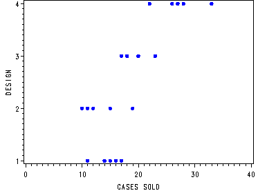
Fig. 16.3, p. 677.

goptions reset=all;
 
symbol1 v=dot c=blue h=.8;
axis1 order=(0 to 40 by 10) label=('CASES SOLD');
axis2 label=(angle=90 'DESIGN');
proc gplot data=food;
  plot design*sales/ haxis=axis1 vaxis=axis2;
run;
quit;

Calculations of SSTO, SSTR and SSE, p. 683 as well as the least squares and maximum
likelihood estimates of the mean sales per store by package design, p. 679. Also included is the F-test, p. 691.

proc glm data=food;
  class design;
  model sales=design;
  means design;
  output out=temp r=resid;
run;
quit;

The GLM Procedure

Class Level Information

Class Levels Values
design 4 1 2 3 4

Number of observations 19

The GLM Procedure

Dependent Variable: sales
Sum of
Source DF Squares Mean Square F Value Pr > F
Model 3 588.2210526 196.0736842 18.59 <.0001
Error 15 158.2000000 10.5466667
Corrected Total 18 746.4210526
R-Square Coeff Var Root MSE sales Mean

0.788055 17.43042 3.247563 18.63158
Source DF Type I SS Mean Square F Value Pr > F
design 3 588.2210526 196.0736842 18.59 <.0001
Source DF Type III SS Mean Square F Value Pr > F
design 3 588.2210526 196.0736842 18.59 <.0001

The GLM Procedure

Level of ————sales————
design N Mean Std Dev
1 5 14.6000000 2.30217289
2 5 13.4000000 3.64691651
3 4 19.5000000 2.64575131
4 5 27.2000000 3.96232255

Table 16.2, p. 680.

proc freq data=temp;
  weight resid;
  tables design*store/ norow nocol nopercent table;
run;

The FREQ Procedure
Table of design by store

design     store
Frequency|       1|       2|       3|       4|       5|  Total

———+——–+——–+——–+——–+——–+

       1 |   -3.6 |    2.4 |    1.4 |   -0.6 |    0.4 | 18E-16

———+——–+——–+——–+——–+——–+

       2 |   -1.4 |   -3.4 |    1.6 |    5.6 |   -2.4 | 71E-16

———+——–+——–+——–+——–+——–+

       3 |    3.5 |    0.5 |   -1.5 |   -2.5 |      0 |      0

———+——–+——–+——–+——–+——–+

       4 |   -0.2 |    5.8 |   -5.2 |   -1.2 |    0.8 | 21E-15

———+——–+——–+——–+——–+——–+

Total        -1.7      5.3     -3.7      1.3     -1.2  302E-16

Coding Indicator variables to be used in the regression version of the Kenton Food example, p. 698.

data foodreg;
  set food;
  x1=0 ;
  if design=1 then x1=1;
  else if design=4 then x1=-1;
  x2=0 ;
  if design=2 then x2=1;
  else if design=4 then x2=-1;
  x3=0 ;
  if design=3 then x3=1;
  else if design=4 then x3=-1;
run;

Table 16.4a, p. 699.

proc print data=foodreg (obs=15);
run;

Obs sales design store x1 x2 x3

1 11 1 1 1 0 0
2 17 1 2 1 0 0
3 16 1 3 1 0 0
4 14 1 4 1 0 0
5 15 1 5 1 0 0
6 12 2 1 0 1 0
7 10 2 2 0 1 0
8 15 2 3 0 1 0
9 19 2 4 0 1 0
10 11 2 5 0 1 0
11 23 3 1 0 0 1
12 20 3 2 0 0 1
13 18 3 3 0 0 1
14 17 3 4 0 0 1
15 27 4 1 -1 -1 -1

Fitting the regression model, table 16.4b and 16.4c, p. 699.

proc reg data=foodreg;
  model sales = x1-x3;
run;
quit;

The REG Procedure
Model: MODEL1
Dependent Variable: sales

Analysis of Variance

Sum of Mean
Source DF Squares Square F Value Pr > F
Model 3 588.22105 196.07368 18.59 <.0001
Error 15 158.20000 10.54667
Corrected Total 18 746.42105

Root MSE 3.24756 R-Square 0.7881
Dependent Mean 18.63158 Adj R-Sq 0.7457
Coeff Var 17.43042
Parameter Estimates

Parameter Standard
Variable DF Estimate Error t Value Pr > |t|
Intercept 1 18.67500 0.74853 24.95 <.0001
x1 1 -4.07500 1.27081 -3.21 0.0059
x2 1 -5.27500 1.27081 -4.15 0.0009
x3 1 0.82500 1.37063 0.60 0.5562