Applied Linear Statistical Models by Neter, Kutner, et. al. Chapter 19: Two-factor Analysis of Variance-Equal Sample Sizes

Inputting the Castle Bakery data, table 19.7, p. 818.

data bakery;
  input sales height width store;
cards;
  47  1  1  1
  43  1  1  2
  46  1  2  1
  40  1  2  2
  62  2  1  1
  68  2  1  2
  67  2  2  1
  71  2  2  2
  41  3  1  1
  39  3  1  2
  42  3  2  1
  46  3  2  2
;
run;

Means for levels of height, width and height by width, table 19.7, p. 818.
Note: Using proc glm to generate the means by using the lsmeans
statement is one of the most convenient ways of obtaining these means.
The alternative would be to use three proc means one for each of the
categorical variables and their interaction. Unfortunately, proc glm
does provide a great deal of output and we have therefore deleted irrelevant
(to this computation) results for the sake of clarity.

proc glm data=bakery;
  class height width;
  model sales = height width height*width;
  lsmeans height width height*width;
run;
quit;

The GLM Procedure

<ouput omittd>

The GLM Procedure
Least Squares Means

height sales LSMEAN
1 44.0000000
2 67.0000000
3 42.0000000
width sales LSMEAN
1 50.0000000
2 52.0000000
height width sales LSMEAN
1 1 45.0000000
1 2 43.0000000
2 1 65.0000000
2 2 69.0000000
3 1 40.0000000
3 2 44.0000000

Fig. 19.6, p. 820.
In order to get the lines on the same graph we need to create two variables for height that corresponds to each of
the levels of width. The overlay option in the plot statement lets us plot both lines in the
same graph.

ods listing close;
proc means data= bakery mean ;
  class height width;
  var sales;
  ods output summary=sum;
run;
ods listing;
ods output close;
data sum;
  set sum;
  if width = 1 then regular=height;
  if width = 2 then wide =height;
run;
goptions reset = all;
 
symbol1 c=blue v=.8 i=join;
symbol2 c=red v=.8 i=join;
axis1 label=( 'Height');
axis2 label=(angle=90 'Sales');
legend1 label=none value=(height=1 font=swiss 'Regular' 'Wide' ) 
        position=( middle bottom inside) mode=share cborder=black;
proc gplot data=sum;
  plot sales_Mean*regular=1 sales_Mean*wide=2 /overlay haxis=axis1 vaxis=axis2 legend=legend1;
run;
quit;

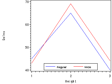
Table 19.9 and Fig. 19.7, p. 820-824.
Note: Unlike in the prior results from table 19.7 here we have kept all the
results from the proc glm because we now would like to examine the
anova table results. We also utilized the output statement in
order to obtain the residual and predicted values in a separate dataset.
We will use these in the graphs in fig. 19.8.

proc glm data=bakery;
  class height width;
  model sales = height width height*width;
  means height width height*width;
  output out=temp r=resid p=predict;
run;
quit;

The GLM Procedure

Class Level Information

Class Levels Values

height 3 1 2 3
width 2 1 2

Number of observations 12
The GLM Procedure

Dependent Variable: sales
Sum of
Source DF Squares Mean Square F Value Pr > F
Model 5 1580.000000 316.000000 30.58 0.0003
Error 6 62.000000 10.333333
Corrected Total 11 1642.000000
R-Square Coeff Var Root MSE sales Mean
0.962241 6.303040 3.214550 51.00000
Source DF Type I SS Mean Square F Value Pr > F
height 2 1544.000000 772.000000 74.71 <.0001
width 1 12.000000 12.000000 1.16 0.3226
height*width 2 24.000000 12.000000 1.16 0.3747
Source DF Type III SS Mean Square F Value Pr > F
height 2 1544.000000 772.000000 74.71 <.0001
width 1 12.000000 12.000000 1.16 0.3226
height*width 2 24.000000 12.000000 1.16 0.3747

The GLM Procedure

Level of ————sales————
height N Mean Std Dev
1 4 44.0000000 3.16227766
2 4 67.0000000 3.74165739
3 4 42.0000000 2.94392029
Level of ————sales————
width N Mean Std Dev
1 6 50.0000000 12.0664825
2 6 52.0000000 13.4313067

Level of Level of ————sales————
height width N Mean Std Dev
1 1 2 45.0000000 2.82842712
1 2 2 43.0000000 4.24264069
2 1 2 65.0000000 4.24264069
2 2 2 69.0000000 2.82842712
3 1 2 40.0000000 1.41421356
3 2 2 44.0000000 2.82842712

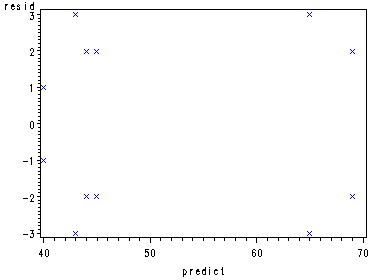
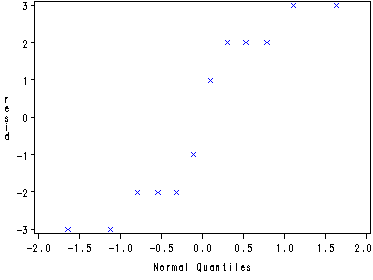
Fig. 19.8, p. 828.

goptions reset=all;

symbol1 v=x c=blue h=.8;
proc gplot data=temp;
  plot resid*predict;
run;
quit;
symbol1 v=x c=blue h=.8;
proc capability data=temp noprint;
  qqplot resid;
run;

F tests of the interaction and main effects, p. 830-831.

proc glm data=bakery;
  class height width;
  model sales = height width height*width;
  run;
quit;

The GLM Procedure

Class Level Information

Class Levels Values
height 3 1 2 3
width 2 1 2

Number of observations 12
The GLM Procedure

Dependent Variable: sales
Sum of
Source DF Squares Mean Square F Value Pr > F
Model 5 1580.000000 316.000000 30.58 0.0003
Error 6 62.000000 10.333333
Corrected Total 11 1642.000000
R-Square Coeff Var Root MSE sales Mean
0.962241 6.303040 3.214550 51.00000
Source DF Type I SS Mean Square F Value Pr > F
height 2 1544.000000 772.000000 74.71 <.0001
width 1 12.000000 12.000000 1.16 0.3226
height*width 2 24.000000 12.000000 1.16 0.3747
Source DF Type III SS Mean Square F Value Pr > F
height 2 1544.000000 772.000000 74.71 <.0001
width 1 12.000000 12.000000 1.16 0.3226
height*width 2 24.000000 12.000000 1.16 0.3747

Creating the dummy and interaction variables for the Regression model of the Bakery data, p. 833.

data dummy;
  set bakery;
  x1=0;
  if height=1 then x1=1;
  if height=3 then x1 = -1;
  x2=0;
  if height=2 then x2=1;
  if height=3 then x2 = -1;
  x3=0;
  if width=1 then x3=1;
  if width=2 then x3 = -1;
  x13 = x1*x3;
  x23 = x2*x3;
run;

Table 19.10, p. 836.
Note: It is the SS1 option in the model statement that supplies the type 1 sums of squares for each predictor.

proc print data=dummy;
run;
proc reg data=dummy;
  model sales = x1 x2 x3 x13 x23 / ss1;
run;
quit;

Obs sales height width store x1 x2 x3 x13 x23
1 47 1 1 1 1 0 1 1 0
2 43 1 1 2 1 0 1 1 0
3 46 1 2 1 1 0 -1 -1 0
4 40 1 2 2 1 0 -1 -1 0
5 62 2 1 1 0 1 1 0 1
6 68 2 1 2 0 1 1 0 1
7 67 2 2 1 0 1 -1 0 -1
8 71 2 2 2 0 1 -1 0 -1
9 41 3 1 1 -1 -1 1 -1 -1
10 39 3 1 2 -1 -1 1 -1 -1
11 42 3 2 1 -1 -1 -1 1 1
12 46 3 2 2 -1 -1 -1 1 1

The REG Procedure
Model: MODEL1
Dependent Variable: sales

Analysis of Variance

Sum of Mean
Source DF Squares Square F Value Pr > F
Model 5 1580.00000 316.00000 30.58 0.0003
Error 6 62.00000 10.33333
Corrected Total 11 1642.00000

Root MSE 3.21455 R-Square 0.9622
Dependent Mean 51.00000 Adj R-Sq 0.9308
Coeff Var 6.30304
Parameter Estimates

Parameter Standard
Variable DF Estimate Error t Value Pr > |t| Type I SS
Intercept 1 51.00000 0.92796 54.96 <.0001 31212
x1 1 -7.00000 1.31233 -5.33 0.0018 8.00000
x2 1 16.00000 1.31233 12.19 <.0001 1536.00000
x3 1 -1.00000 0.92796 -1.08 0.3226 12.00000
x13 1 2.00000 1.31233 1.52 0.1783 18.00000
x23 1 -1.00000 1.31233 -0.76 0.4749 6.00000

Pooling sums of squares in the Bakery Sales example, p. 837.
Note: The change in the SSE has been italicized for clarity.

proc glm data=dummy;
  class height width;
  model sales = height width;
run;
quit;

The GLM Procedure

Class Level Information

Class Levels Values
height 3 1 2 3
width 2 1 2

Number of observations 12
The GLM Procedure

Dependent Variable: sales
Sum of
Source DF Squares Mean Square F Value Pr > F
Model 3 1556.000000 518.666667 48.25 <.0001
Error 8 86.000000 10.750000
Corrected Total 11 1642.000000
R-Square Coeff Var Root MSE sales Mean
0.947625 6.428861 3.278719 51.00000

Source DF Type I SS Mean Square F Value Pr > F
height 2 1544.000000 772.000000 71.81 <.0001
width 1 12.000000 12.000000 1.12 0.3216
Source DF Type III SS Mean Square F Value Pr > F
height 2 1544.000000 772.000000 71.81 <.0001
width 1 12.000000 12.000000 1.12 0.3216