Applied Linear Statistical Models by Neter, Kutner, et. al. Chapter 11: Qualitative Predictor Variables

Inputting the Insurance Innovation Data, Table 11.1, p. 459.

data ch11tab01;
  input y x1 x2;
  label  y = 'Months'
        x1 = 'Size'
	x2 = 'Firm Indicator';
cards;
  17  151  0
  26   92  0
  21  175  0
  30   31  0
  22  104  0
   0  277  0
  12  210  0
  19  120  0
   4  290  0
  16  238  0
  28  164  1
  15  272  1
  11  295  1
  38   68  1
  31   85  1
  21  224  1
  20  166  1
  13  305  1
  30  124  1
  14  246  1
;
run;

Table 11.2, p. 459.

proc reg data = ch11tab01;
  model y = x1 x2/ clb;
run;
quit;

The REG Procedure
Model: MODEL1
Dependent Variable: y Months

                             Analysis of Variance

                                    Sum of           Mean
Source                   DF        Squares         Square    F Value    Pr > F

Model                     2     1504.41333      752.20667      72.50    <.0001
Error                    17      176.38667       10.37569
Corrected Total          19     1680.80000


Root MSE              3.22113    R-Square     0.8951
Dependent Mean       19.40000    Adj R-Sq     0.8827
Coeff Var            16.60377

                                 Parameter Estimates

                                       Parameter       Standard
Variable     Label             DF       Estimate          Error    t Value    Pr > |t|

Intercept    Intercept          1       33.87407        1.81386      18.68      <.0001
x1           Size               1       -0.10174        0.00889     -11.44      <.0001
x2           Firm Indicator     1        8.05547        1.45911       5.52      <.0001

                      Parameter Estimates

Variable     Label             DF       95% Confidence Limits

Intercept    Intercept          1       30.04716       37.70098
x1           Size               1       -0.12050       -0.08298
x2           Firm Indicator     1        4.97703       11.13391

Fig. 11.2, p. 460.

data ch11tab01;
  set ch11tab01;
  if x2 = 0 then do;
  z1 = x1;
  y1 = y;
  end;
  if x2= 1 then do;
  z2 = x1 ;
  y2 = y;
  end;
run;
proc reg data = ch11tab01 noprint;
  model y = z1 ;
  output out = temp1 p = p1;
run;
proc reg data = temp1 noprint;
  model y = z2;
  output out=temp p= p2;
run;
quit;
 
symbol1 c=red v=circle;
symbol2 c=blue v=dot i=none;
symbol3 i=join v=none c=red;
symbol4 i=join v=none c=blue;
axis1 order=(0 to 350 by 50)label=('Size of Firm');
axis2 label=(angle = 90 'Months Elapsed');
proc gplot data = temp;
  plot y1*z1  y2*z2 p1*z1 p2*z2 / overlay haxis = axis1 vaxis=axis2;
run;
quit;

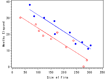
Table 11.3, p. 464.
Note: First create the interaction variable and then run the regression.

data ch11tab01;
  set ch11tab01;
  x1x2 = x1*x2;
run;
proc reg data = ch11tab01;
  model y = x1 x2 x1x2;
run;
quit;

The REG Procedure
Model: MODEL1
Dependent Variable: y Months

Analysis of Variance

Sum of Mean
Source DF Squares Square F Value Pr > F

Model 3 1504.41904 501.47301 45.49 <.0001
Error 16 176.38096 11.02381
Corrected Total 19 1680.80000

Root MSE 3.32021 R-Square 0.8951
Dependent Mean 19.40000 Adj R-Sq 0.8754
Coeff Var 17.11450

Parameter Estimates

Parameter Standard
Variable Label DF Estimate Error t Value Pr > |t|

Intercept Intercept 1 33.83837 2.44065 13.86 <.0001
x1 Size 1 -0.10153 0.01305 -7.78 <.0001
x2 Firm Indicator 1 8.13125 3.65405 2.23 0.0408
x1x2 1 -0.00041714 0.01833 -0.02 0.9821

Inputting the Soap Production data, table 11.4, p. 469.

data ch11tab04;
  input y x1 x2;
  label  y = 'Scrap'
        x1 = 'Speed'
	x2 = 'Production line';
cards;
  218  100  1
  248  125  1
  360  220  1
  351  205  1
  470  300  1
  394  255  1
  332  225  1
  321  175  1
  410  270  1
  260  170  1
  241  155  1
  331  190  1
  275  140  1
  425  290  1
  367  265  1
  140  105  0
  277  215  0
  384  270  0
  341  255  0
  215  175  0
  180  135  0
  260  200  0
  361  275  0
  252  155  0
  422  320  0
  273  190  0
  410  295  0
;
run;

Fig. 11.6, p. 470.

goption reset=all;
symbol1 c=red v=circle;
symbol2 c=blue v=dot;
axis1 order=(100 to 350 by 50);
proc gplot data = ch11tab04;
  plot y*x1 = x2 / haxis = axis1;
run;
quit;

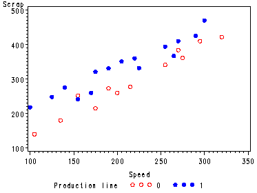
Table 11.5, p. 471.
The test is the F-test (11.19) p. 472-473. The clb option in the model statement
gives us confidence intervals including the CI for beta2 at the bottom of p. 473.
Note1: First create the interaction term, then run the regression.
Note2: The residuals and the fitted values where outputted to be used in Fig. 11.5.

data ch11tab04;
  set ch11tab04;
  x1x2 = x1*x2;
run;
proc reg data = ch11tab04;
  model y = x1 x2 x1x2/ ss1 clb;
  output out=temp p=yhat r=residual;
  test: test x2=x1x2=0;
run;
quit;

The REG Procedure
Model: MODEL1
Dependent Variable: y Scrap

Analysis of Variance

Sum of Mean
Source DF Squares Square F Value Pr > F

Model 3 169165 56388 130.95 <.0001
Error 23 9904.05692 430.61117
Corrected Total 26 179069

Root MSE 20.75117 R-Square 0.9447
Dependent Mean 315.48148 Adj R-Sq 0.9375
Coeff Var 6.57762

Parameter Estimates

Parameter Standard
Variable Label DF Estimate Error t Value Pr > |t| Type I SS

Intercept Intercept 1 7.57446 20.86970 0.36 0.7200 2687271
x1 Speed 1 1.32205 0.09262 14.27 <.0001 149661
x2 Production line 1 90.39086 28.34573 3.19 0.0041 18694
x1x2 1 -0.17666 0.12884 -1.37 0.1835 809.62258

Parameter Estimates

Variable Label DF 95% Confidence Limits

Intercept Intercept 1 -35.59779 50.74672
x1 Speed 1 1.13044 1.51366
x2 Production line 1 31.75325 149.02848
x1x2 1 -0.44318 0.08986

The REG Procedure
Model: MODEL1

Test test Results for Dependent Variable y

Mean
Source DF Square F Value Pr > F

Numerator 2 9751.85064 22.65 <.0001
Denominator 23 430.61117

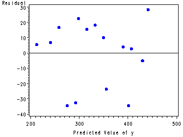
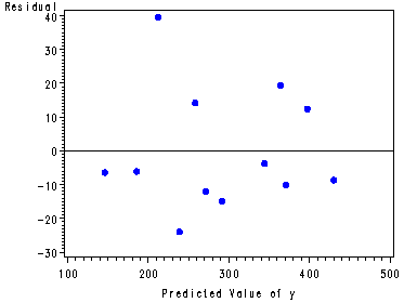
Fig. 11.5a and 11.5b, p. 471.

proc sort data = temp;
by x2;
run;
symbol1 c=blue v=dot;
proc gplot data = temp;
  by x2;
  plot residual*yhat/ vref = 0;
run;
quit;

Inputting the Lot Size data, table 11.6, p. 477.
Creating the x2 and (x1-500)*x2 variables.

data ch11tab06 ;
  input y x1;
  label  y = 'Cost'
        x1 = 'Lot Size';
cards;
  2.57  650
  4.40  340
  4.52  400
  1.39  800
  4.75  300
  3.55  570
  2.49  720
  3.77  480
;
run;
data ch11tb06a;
  set ch11tab06;
  x2 = .;
  if x1 > 500 then x2 = 1; 
    else x2 = 0;
  x3 = (x1 - 500)*x2;
run;

The regression model at the bottom of p. 476.
Note: x3 = (x1-500)*x2.

proc reg data = ch11tb06a;
  model y = x1 x3;
  output out=temp p=yhat;
run;
quit;

The REG Procedure
Model: MODEL1
Dependent Variable: y Cost

Analysis of Variance

Sum of Mean
Source DF Squares Square F Value Pr > F

Model 2 9.48623 4.74311 79.06 0.0002
Error 5 0.29997 0.05999
Corrected Total 7 9.78620

Root MSE 0.24494 R-Square 0.9693
Dependent Mean 3.43000 Adj R-Sq 0.9571
Coeff Var 7.14106

Parameter Estimates

Parameter Standard
Variable Label DF Estimate Error t Value Pr > |t|

Intercept Intercept 1 5.89545 0.60421 9.76 0.0002
x1 Lot Size 1 -0.00395 0.00149 -2.65 0.0454
x3 1 -0.00389 0.00231 -1.69 0.1528

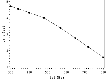
Fig. 11.9, p. 476.

proc sort data = temp;
  by x1;
run;
 
symbol1 i=join c=black v=dot ;
axis1 label=(angle=90 'Unit Cost');
proc gplot data = temp;
  plot yhat*x1/ vaxis=axis1;
run;
quit;

Inputting the AADT Data, Table 11.7, p. 484.

data ch11tab07;
  input y x1 x2 x3 x4 class truck locale;
cards;
    1616   13404  2  52  2  2  5  1
    1329   52314  2  60  2  2  5  1
    3933   30982  2  57  2  4  5  2
    3786   25207  2  64  2  4  5  2
     465   20594  2  40  2  2  5  1
     794   11507  2  44  2  2  5  1
     618    9379  2  43  2  2  5  1
    1150   24991  2  42  2  2  5  1
    1538   30982  2  59  2  2  5  1
    1769   24991  2  41  2  2  5  1
    1304    9379  2  30  2  2  5  1
    4331   25187  4  52  2  4  5  2
   13100  108161  2  48  2  4  5  2
    2538   25717  2  24  2  2  5  1
     420   14098  2  24  2  2  5  1
     429   19871  2  22  2  2  5  1
     399   34844  2  22  2  2  5  1
     201   14773  2  22  2  2  5  1
     587   41722  2  22  2  2  5  1
     384   14854  2  24  2  2  5  1
   20816   36329  4  24  1  1  1  1
   28998  222229  4  24  1  3  1  3
   34317  222229  4  26  1  3  1  3
   23887  222229  4  24  1  3  1  3
   18180  222229  4  24  2  4  2  3
    6410  222229  4  24  2  2  2  1
    3769   43069  2  24  2  2  2  1
   10193   49327  4  24  2  2  1  1
   12808  108161  4  24  1  1  1  1
    1276   25207  2  20  2  2  4  1
   11755   25187  4  24  2  2  2  1
   16567   92006  4  24  2  2  2  1
   19642   25717  4  24  1  1  1  1
   11824   46256  4  24  1  1  1  1
    2934   12361  4  24  2  2  2  1
    1853   20401  2  24  2  2  1  1
    1227   11690  2  24  2  2  2  1
   21582   58681  4  24  1  1  1  1
    5818   18430  2  20  2  2  5  1
    1179   34844  2  24  2  2  2  1
   15734   30328  4  24  1  1  1  1
     680   34844  2  22  2  2  5  1
     877   30982  2  24  2  2  5  1
    2795  222229  2  24  2  2  4  1
   10647   92006  4  24  2  2  1  1
    4933   13043  4  24  2  2  1  1
    1193   21050  2  24  2  2  5  1
     712    7716  2  24  2  2  2  1
     647   12920  2  24  2  2  5  1
    2421   43069  2  24  2  2  2  1
    1669   14098  2  24  2  2  5  1
    1811   14098  2  24  2  2  2  1
    1505   13404  2  24  2  2  4  1
    2417   21050  2  24  2  2  2  1
    1794   20594  2  22  2  2  2  1
     429   52314  2  24  2  2  5  1
    5697   36329  4  24  1  1  1  1
  123665  459784  8  48  1  3  1  3
  105844  941411  6  36  1  3  1  3
   90807  459784  6  36  1  3  1  3
   39799  194279  4  24  1  3  1  2
  123445  941411  6  36  1  3  1  3
   78343  941411  5  36  1  4  5  3
  155547  941411  6  36  1  3  1  3
  139309  941411  6  36  1  3  1  2
   90594  941411  4  24  1  3  1  2
   87003  941411  4  50  1  3  1  3
   61617  459784  4  38  1  3  1  3
   85393  941411  4  24  1  3  1  3
   22165  195998  4  24  1  3  1  2
   36977  194279  6  39  1  3  1  2
   54941  941411  4  24  1  3  1  2
   33272  113571  4  24  1  3  1  2
    4348  194279  2  24  2  2  4  1
    9025  941411  2  24  2  2  2  1
   18574  195998  4  24  2  4  2  2
   12665   43784  4  24  2  2  2  1
   40642  113571  6  36  1  1  1  1
   19341  194279  4  64  2  4  3  2
   40602  941411  4  26  2  4  1  2
   16550  459784  4  24  2  4  5  2
   20240  941411  4  48  2  4  2  2
   28793  195998  4  38  2  4  4  2
   25114  195998  4  24  2  4  2  2
   19007  941411  4  24  2  4  5  2
   23557  194279  4  24  2  4  4  2
    4860   37046  2  24  2  2  2  1
   13823  194279  4  24  2  2  2  1
    8972  113571  2  24  2  2  5  1
    4307  113571  2  24  2  2  5  1
   38857  113571  4  24  2  4  1  1
   12230   25717  2  24  2  2  4  1
     756  941411  2  24  2  2  5  1
    2769  459784  2  44  2  4  5  2
   21961  941411  4  28  2  4  5  2
    9843  941411  4  44  2  4  5  3
   15334  941411  2  24  2  4  5  2
   14975  459784  2  24  2  4  5  2
    1462  194279  2  24  2  2  5  1
    1951   43784  2  22  2  2  5  1
   25426  459784  4  19  2  4  5  2
   44585  941411  4  28  2  4  5  2
   24413  194279  4  26  2  4  5  2
    7494  195998  2  25  2  4  5  2
   17388  194279  4  48  2  4  5  2
     812  194279  2  22  2  2  5  1
    3797   43784  2  49  2  4  5  2
    4312  113571  2  24  2  2  5  1
    1440  113571  2  24  2  2  5  2
   12865  459784  2  50  2  4  5  2
    5626  459784  2  36  2  4  5  3
    3644  459784  2  30  2  4  5  3
    8666  195998  4  44  2  4  5  2
    3317   37046  2  24  2  4  5  2
    4796  194279  2  34  2  4  5  2
    5576  194279  2  40  2  4  5  2
   13723  941411  2  44  2  4  5  2
   21535  941411  4  60  2  4  5  3
   14905  459784  4  68  2  4  5  2
   15408  459784  2  40  2  4  5  3
    1266   43784  2  44  2  4  5  2
;
run;
data ch11tab07;
  set ch11tab07;
  class1 = 0 ;
  if class = 1 then class1 = 1;
  class2 = 0;
  if class = 2 then class2 = 1;
  class3 = 0;
  if class = 3 then class3 = 1;
  truck1 = 0;
  if truck = 1 then truck1 = 1;
  truck2 = 0;
  if truck = 2 then truck2 = 1;
  truck3 = 0;
  if truck = 3 then truck3 = 1;
  truck4 = 0;
  if truck = 4 then truck4 = 1;
  locale1 = 0;
  if locale = 1 then locale1 = 1;
  locale2 = 0;
  if locale = 2 then locale2 = 1;
  label  x1 = 'ctypop'
         x2 = 'lanes'
	 x3 = 'width'
	 x4 = 'control'
     class1 = 'rural int.'
     class2 = 'rural nonint.'
     class3 = 'urban int.'
    locale1 = 'rural'
    locale2 = 'urban <= 50000';
run;

Fig. 11.11, p. 485.
We omit the example of the scatterplot matrix.

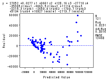
Initial analysis: regression with all the predictors, residual plot, vif’s, the largest
cook’s d.

symbol1 v=dot c=blue h=.8; 
proc reg data = ch11tab07;
  model y = x1-x4 class1 class2 class3 truck1 truck2 truck3 truck4 locale1 locale2/ vif ;
  plot r.*p.;
  output out = temp cookd = cookd;
run;
quit;
proc print data = temp;
  where cookd > 0.05;
  var cookd;
run;

The REG Procedure
Model: MODEL1
Dependent Variable: y

Analysis of Variance

Sum of Mean
Source DF Squares Square F Value Pr > F

Model 13 90306217767 6946632136 38.29 <.0001
Error 107 19409611507 181398238
Corrected Total 120 1.097158E11

Root MSE 13468 R-Square 0.8231
Dependent Mean 19438 Adj R-Sq 0.8016
Coeff Var 69.29022

Parameter Estimates

Parameter Standard Variance
Variable Label DF Estimate Error t Value Pr > |t| Inflation

Intercept Intercept 1 27052 29820 0.91 0.3664 0
x1 ctypop 1 0.02771 0.00496 5.58 <.0001 1.76731
x2 lanes 1 9660.98727 1568.49966 6.16 <.0001 2.75058
x3 width 1 128.15518 129.37566 0.99 0.3241 1.47333
x4 control 1 -27710 14571 -1.90 0.0599 24.54914
class1 rural int. 1 -35365 18298 -1.93 0.0559 13.79023
class2 rural nonint. 1 -6663.52080 10181 -0.65 0.5142 17.18991
class3 urban int. 1 11114 15464 0.72 0.4739 20.19940
truck1 1 -2215.34880 6656.19022 -0.33 0.7399 5.74874
truck2 1 -2659.88513 3985.04860 -0.67 0.5059 1.46150
truck3 1 -1799.71245 14179 -0.13 0.8992 1.09908
truck4 1 5193.99138 5555.04832 0.94 0.3519 1.12192
locale1 rural 1 10927 11133 0.98 0.3286 20.60071
locale2 urban <= 50000 1 -2719.67482 4527.06574 -0.60 0.5493 2.98603

Obs cookd

24 0.05619
64 0.15665
65 0.15316
70 0.05289
71 0.09742
91 0.20761
96 0.07146
109 0.20761

Subset selection: based on Rsquare.
The include option in the model statement will ensure that all models will
include predictors x1 and x2.

proc reg data = ch11tab07;
  model y = x1-x4 class1 class2 class3 truck1 truck2 truck3 truck4 locale1 locale2/
            selection = rsquare cp best = 5 include=2 start = 3 stop = 7;
run;
quit;

The REG Procedure
Model: MODEL1
Dependent Variable: y

R-Square Selection Method

NOTE: The variables in the 2 variable model are included in all models.

Number in
Model R-Square C(p) Variables in Model

2 0.6946 69.7231 x1 x2
————————————————————————————————–
3 0.8045 5.2315 class3
3 0.7514 37.3903 x4
3 0.7258 52.8725 truck1
3 0.7045 65.7318 locale2
3 0.7042 65.8798 class1
————————————————————————————————–
4 0.8121 2.6490 x4 class1
4 0.8104 3.6986 class3 locale2
4 0.8080 5.1275 class3 locale1
4 0.8071 5.6590 class2 class3
4 0.8063 6.1562 class3 truck4
————————————————————————————————–
5 0.8162 2.1414 x4 class1 locale2
5 0.8158 2.3848 x4 class1 locale1
5 0.8144 3.2803 x4 class1 class2
5 0.8139 3.5589 x4 class1 truck4
5 0.8128 4.2321 x4 class1 truck2
————————————————————————————————–
6 0.8183 2.8958 x3 x4 class1 locale1
6 0.8180 3.0845 x4 class1 truck4 locale2
6 0.8179 3.1309 x4 class1 truck2 locale2
6 0.8177 3.2367 x4 class1 truck2 locale1
6 0.8177 3.2383 x3 x4 class1 locale2
————————————————————————————————–
7 0.8204 3.6023 x3 x4 class1 truck4 locale1
7 0.8199 3.9050 x3 x4 class1 truck4 locale2
7 0.8195 4.1891 x3 x4 class1 truck2 locale1
7 0.8192 4.3663 x4 class1 truck2 truck4 locale2
7 0.8190 4.4705 x3 x4 class1 class2 locale1

Analyzing the model consisting of the predictors:
x1, x2, x4, class1 and class3.
If you would like to run proc rsquare this is still possible in SAS v. 8 but it
might be hard to find help for this procedure. It might be easier to use the
selection = rsquare option in proc reg which will produce the same results.

symbol1 v=dot c=blue h=.8;
proc reg data = ch11tab07;
  model y = x1 x2 x4 class1 class3;
  plot student.*p.;
run;
quit;

The Studentized Residual plot is fig. 11.13a, p. 487.

blockquote>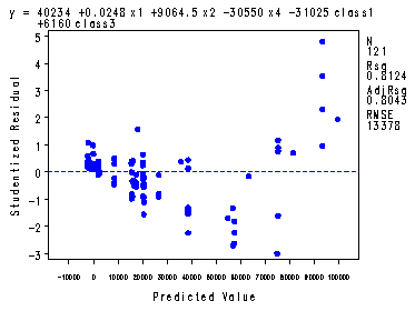

The REG Procedure
Model: MODEL1
Dependent Variable: y

Analysis of Variance

Sum of Mean
Source DF Squares Square F Value Pr > F

Model 5 89135575295 17827115059 99.62 <.0001
Error 115 20580253979 178958730
Corrected Total 120 1.097158E11

Root MSE 13378 R-Square 0.8124
Dependent Mean 19438 Adj R-Sq 0.8043
Coeff Var 68.82273

Parameter Estimates

Parameter Standard
Variable Label DF Estimate Error t Value Pr > |t|

Intercept Intercept 1 40234 28710 1.40 0.1638
x1 ctypop 1 0.02479 0.00436 5.68 <.0001
x2 lanes 1 9064.52332 1329.74878 6.82 <.0001
x4 control 1 -30550 13960 -2.19 0.0307
class1 rural int. 1 -31025 14661 -2.12 0.0365
class3 urban int. 1 6160.03616 13835 0.45 0.6570

Investigating curvilinearity: considering squared terms of x1 and x2, interactions and
running the model selection procedure again with all the new variables included.
Note: The variables x1 and x2 should be centered first!

proc means data = ch11tab07;
  var x1 x2;
  output out=mout mean=mx1 mx2;
run;
data center;
  if _n_ = 1 then set mout;
  set ch11tab07;
  cx1 = x1 - mx1;
  cx2 = x2 - mx2;
run;
data center;
  set center;
  x1sq = cx1**2;
  x2sq = cx2**2;
  x1x2 = cx1*cx2;
  x1x4 = cx1*x4;
  x2x4 = cx2*x4;
  x1c1 = cx1*class1;
  x1c2 = cx1*class2;
  x2c1 = cx2*class1;
  x2c2 = cx2*class2;
  x4c1 = x4*class1;
  x4c2 = x4*class2;
run;
proc reg data = center;
  model y = x1 x2 x4 class1 class2 x1sq x2sq x1x2 x1x4 x2x4 x1c1 x1c2 x2c1 x2c2 x4c1 x4c2/
            selection =rsquare cp include=2 start=3 stop = 7 best = 5;
run;
quit;

The MEANS Procedure

Variable Label N Mean Std Dev Minimum Maximum
—————————————————————————————–
x1 ctypop 121 263427.67 329469.96 7716.00 941411.00
x2 lanes 121 3.0991736 1.3000318 2.0000000 8.0000000
—————————————————————————————–

The REG Procedure
Model: MODEL1
Dependent Variable: y

R-Square Selection Method

NOTE: The variables in the 2 variable model are included in all models.

Number in
Model R-Square C(p) Variables in Model

2 0.6946 388.0053 x1 x2
————————————————————————————————–
3 0.8748 93.2202 x1x4
3 0.8283 169.7793 x2x4
3 0.8203 182.9602 x1x2
3 0.7657 272.9252 x2sq
3 0.7514 296.5162 x4
————————————————————————————————–
4 0.9231 15.6875 x1x4 x2x4
4 0.9010 52.1299 x2sq x1x4
4 0.8977 57.4939 x4 x1x4
4 0.8857 77.3097 x1x4 x2c2
4 0.8835 80.9151 x1x2 x1x4
————————————————————————————————–
5 0.9281 9.3483 class2 x1x4 x2x4
5 0.9281 9.3483 x1x4 x2x4 x4c2
5 0.9253 13.9612 x1x2 x1x4 x2x4
5 0.9246 15.2330 x4 x2sq x1x4
5 0.9244 15.4813 x1sq x1x4 x2x4
————————————————————————————————–
6 0.9313 6.0695 class2 x1x2 x1x4 x2x4
6 0.9313 6.0695 x1x2 x1x4 x2x4 x4c2
6 0.9299 8.4143 class2 x1x4 x2x4 x2c1
6 0.9299 8.4143 x1x4 x2x4 x2c1 x4c2
6 0.9293 9.4977 class2 x1x4 x2x4 x2c2
————————————————————————————————–
7 0.9331 5.2325 x4 class2 x2sq x1x2 x1x4
7 0.9331 5.2325 x4 x2sq x1x2 x1x4 x4c2
7 0.9324 6.3338 class2 x1x2 x1x4 x2x4 x2c1
7 0.9324 6.3338 x1x2 x1x4 x2x4 x2c1 x4c2
7 0.9322 6.5830 x4 x1sq x2sq x1x2 x1x4

NOTE: Models of not full rank are not included.

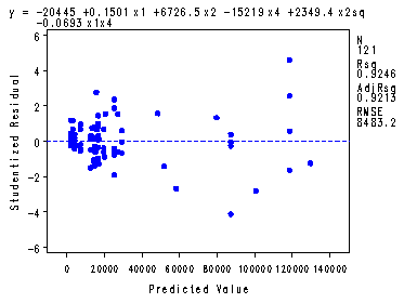
Looking at the best model consisting of x1, x2, x4,
x2sq and x1x4, studentized residual plot, cook’s d, vif’s.
The Studentized Residual plot is Fig. 11.13b, p. 487.

 
symbol1 v=dot c=blue h=.8;
 
proc reg data = center;
  model y = x1 x2 x4 x2sq x1x4/vif;
  plot student.*p.;
  output out = temp cookd = cookd r=r;
run;
quit;
proc print data = temp;
  where cookd > .3;
  var cookd;
run;

The REG Procedure
Model: MODEL1
Dependent Variable: y

Analysis of Variance

Sum of Mean
Source DF Squares Square F Value Pr > F

Model 5 1.014399E11 20287971900 281.91 <.0001
Error 115 8275969776 71964955
Corrected Total 120 1.097158E11

Root MSE 8483.21605 R-Square 0.9246
Dependent Mean 19438 Adj R-Sq 0.9213
Coeff Var 43.64314

Parameter Estimates

Parameter Standard Variance
Variable Label DF Estimate Error t Value Pr > |t| Inflation

Intercept Intercept 1 -20445 7409.59780 -2.76 0.0067 0
x1 ctypop 1 0.15006 0.00942 15.92 <.0001 16.07236
x2 lanes 1 6726.51683 946.81627 7.10 <.0001 2.52639
x4 control 1 -15219 2536.25608 -6.00 <.0001 1.87487
x2sq 1 2349.44748 367.04996 6.40 <.0001 1.63001
x1x4 1 -0.06926 0.00542 -12.79 <.0001 15.49519
Obs cookd

58 0.46168
64 0.47268
72 0.45639

Weighted LS Analysis: using a standard deviation function, p.
486-488, Fig. 11.14.

We have skipped this example.

Table 11.8 was not reproduced.