Applied Linear Statistical Models by Neter, Kutner, et. al. Chapter 13: Introduction to Nonlinear Regression

options nodate nocenter;

Inputting the Severely Injured Patients data, table 13.1, p. 536.

data ch13tab01;
  input y x;
  label x = 'Days'
        y = 'Prognosis';
cards;
  54   2
  50   5
  45   7
  37  10
  35  14
  25  19
  20  26
  16  31
  18  34
  13  38
   8  45
  11  52
   8  53
   4  60
   6  65
;;;
run;

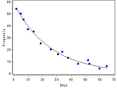
Fig. 13.2, p. 537.

data ch13tab01;
  set ch13tab01;
  yhat = 58.6065*exp(-0.03959*x);
run; 
 
symbol1 v = dot c=blue;
symbol2 i=join c=black v=none;
axis1 label = ( angle = 90 h=1)  ;
proc gplot data = ch13tab01;
  plot y*x yhat*x/overlay vaxis=axis1;
run;
quit;
goptions reset=all;

Getting the starting parameter values from the linear regression, p. 543.

data ch13tab01;
  set ch13tab01;
  yprime = log(y);
run;
proc reg data = ch13tab01;
  model yprime = x;
run;
quit;

The REG Procedure
Model: MODEL1
Dependent Variable: yprime

Analysis of Variance

Sum of Mean
Source DF Squares Square F Value Pr > F

Model 1 8.89295 8.89295 276.38 <.0001
Error 13 0.41830 0.03218
Corrected Total 14 9.31125

Root MSE 0.17938 R-Square 0.9551
Dependent Mean 2.87009 Adj R-Sq 0.9516
Coeff Var 6.24994

Parameter Estimates

Parameter Standard
Variable Label DF Estimate Error t Value Pr > |t|

Intercept Intercept 1 4.03716 0.08410 48.00 <.0001
x Days 1 -0.03797 0.00228 -16.62 <.0001

Table 13.3, p. 545. Using the Gauss-Newton method to get the nonlinear regression estimates.

proc nlin data = ch13tab01 method = newton;
  parms g0=56.6646 g1=-0.03797;
  model y = g0*exp(g1*x);
  output out=temp r=residual p=fitted;
run;

The NLIN Procedure
Iterative Phase
Dependent Variable y
Method: Newton

Sum of
Iter g0 g1 Squares

0 56.6646 -0.0380 56.0867
1 58.5566 -0.0395 49.4641
2 58.6065 -0.0396 49.4593
3 58.6066 -0.0396 49.4593

NOTE: Convergence criterion met.

Estimation Summary

Method Newton
Iterations 3
R 3.56E-11
PPC 5.37E-12
RPC(g1) 2.016E-6
Object 1.62E-10
Objective 49.4593
Observations Read 15
Observations Used 15
Observations Missing 0

NOTE: An intercept was not specified for this model.

Sum of Mean Approx
Source DF Squares Square F Value Pr > F

Regression 2 12060.5 6030.3 1585.01 <.0001
Residual 13 49.4593 3.8046
Uncorrected Total 15 12110.0

Corrected Total 14 3943.3

Approx
Parameter Estimate Std Error Approximate 95% Confidence Limits

g0 58.6066 1.4845 55.3995 61.8136
g1 -0.0396 0.00174 -0.0433 -0.0358

The NLIN Procedure

Approximate Correlation Matrix
g0 g1

g0 1.0000000 -0.7129787
g1 -0.7129787 1.0000000

Fig. 13.3a, p. 549.

 
symbol1 v=dot c=blue;
axis1 label=(angle=90 h=1);
proc gplot data = temp;
  plot residual*fitted /vref = 0 vaxis = axis1;
run;
quit;
goptions reset=all;

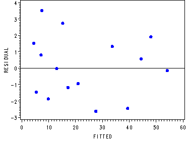
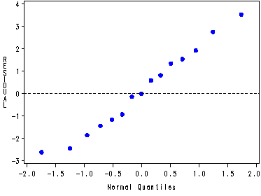
Fig. 13.3b, p. 549.

 
symbol1 v=dot c=blue; 
proc capability data=temp noprint;
  qqplot residual / vref = 0;
run;
goptions reset=all;

Inputting the Learning curve data, table 13.4, p. 556.

data ch13tab04;
  input x1 x2 y;
  label x1 = 'Location'
        x2 = 'Week'
	y = 'Efficiency';
cards;
  1   1   .483
  1   2   .539
  1   3   .618
  1   5   .707
  1   7   .762
  1  10   .815
  1  15   .881
  1  20   .919
  1  30   .964
  1  40   .959
  1  50   .968
  1  60   .971
  1  70   .960
  1  80   .967
  1  90   .975
  0   1   .517
  0   2   .598
  0   3   .635
  0   5   .750
  0   7   .811
  0  10   .848
  0  15   .943
  0  20   .971
  0  30  1.012
  0  40  1.015
  0  50  1.007
  0  60  1.022
  0  70  1.028
  0  80  1.017
  0  90  1.023
;;;
run;

Fig. 13.5, p. 556.

data ch13tab04;
  set ch13tab04;
  if x1 = 0 then do;
  y1 = y;
  z21 = x2;
  p1 = 1.0156 - 0.5524*exp(-0.1348*z21);
  end;
  if x1 = 1 then do;
  y2 = y;
  z22 = x2;
  p2 = 0.9683 - 0.5524*exp(-0.1348*z22);
  end;
run;
  
symbol1 c=red v=circle;
symbol2 c=blue v=dot;
symbol3 i=join v=none c=red;
symbol4 i=join v=none c=blue;
axis1 label = (angle = 90 'Relative Efficiency');
axis2 label = ( 'Time (Week)');
 
legend1 label=none value=(height=1 font=swiss 'Locale A' 'Locale B' 'Fitted Reg Line'
                          'Fitted Reg Line') 
        position=(bottom right inside) mode=share cborder=black;
 
proc gplot data = ch13tab04;
  plot y1*z21 y2*z22 p1*z21 p2*z22 / overlay vaxis= axis1 haxis=axis2 legend=legend1;
run;
quit;
goptions reset=all;

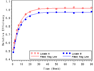
Table 13.5, p. 557 and the confidence interval for gamma1, p. 558.
Note: In the formula the gamma2 and gamma3 are switched compared to the results in table 13.5.

proc nlin data = ch13tab04 method = newton;
  parms g0=1.025 g1=-0.0459 g2=-0.5 g3=-0.122 ;
  model y = g0 + g1*x1 + g2*exp(g3*x2);
run;

The NLIN Procedure
Iterative Phase
Dependent Variable y
Method: Newton
Sum of
Iter g0 g1 g2 g3 Squares

0 1.0250 -0.0459 -0.5000 -0.1220 0.0160
1 1.0158 -0.0473 -0.5466 -0.1325 0.00336
2 1.0156 -0.0473 -0.5524 -0.1347 0.00329
3 1.0156 -0.0473 -0.5524 -0.1348 0.00329

NOTE: Convergence criterion met.

Estimation Summary

Method Newton
Iterations 3
R 1.003E-6
PPC(g3) 1.671E-7
RPC(g3) 0.000356
Object 5.005E-6
Objective 0.003293
Observations Read 30
Observations Used 30
Observations Missing 0

Sum of Mean Approx
Source DF Squares Square F Value Pr > F

Regression 4 22.8541 5.7135 2272.64 <.0001
Residual 26 0.00329 0.000127
Uncorrected Total 30 22.8574

Corrected Total 29 0.8667

Approx
Parameter Estimate Std Error Approximate 95% Confidence Limits

g0 1.0156 0.00369 1.0080 1.0232
g1 -0.0473 0.00411 -0.0557 -0.0388
g2 -0.5524 0.00825 -0.5694 -0.5355
g3 -0.1348 0.00452 -0.1441 -0.1255

The NLIN Procedure

Approximate Correlation Matrix
g0 g1 g2 g3

g0 1.0000000 -0.5560826 -0.1247886 0.4236608
g1 -0.5560826 1.0000000 0.0000000 0.0000000
g2 -0.1247886 0.0000000 1.0000000 0.5741495
g3 0.4236608 0.0000000 0.5741495 1.0000000

For more in-depth information and examples of nonlinear regression in SAS please visit our
web page: Nonlinear regression in SAS
in the Library section of our SAS webpage.