Applied Linear Statistical Models by Neter, Kutner, et. al. Chapter 2: Inferences in Regression Analysis

Inputting the Toluca Company data.

data ch1tab01;
  input x y;
  label x = 'Lot Size'
        y = 'Work Hrs';
cards;
   80  399
   30  121
   50  221
   90  376
   70  361
   60  224
  120  546
   80  352
  100  353
   50  157
   40  160
   70  252
   90  389
   20  113
  110  435
  100  420
   30  212
   50  268
   90  377
  110  421
   30  273
   90  468
   40  244
   80  342
   70  323
;
run;

Table 2.1 and Fig. 2.2, p. 50-51.

proc reg data = ch1tab01;
  model y = x/ clb;
run;
quit;

The REG Procedure
Model: MODEL1
Dependent Variable: y Work Hrs

Analysis of Variance

Sum of Mean
Source DF Squares Square F Value Pr > F

Model 1 252378 252378 105.88 <.0001
Error 23 54825 2383.71562
Corrected Total 24 307203

Root MSE 48.82331 R-Square 0.8215
Dependent Mean 312.28000 Adj R-Sq 0.8138
Coeff Var 15.63447

Parameter Estimates

Parameter Standard
Variable Label DF Estimate Error t Value Pr > |t| 95% Confidence Limits

Intercept Intercept 1 62.36586 26.17743 2.38 0.0259 8.21371 116.51801
x Lot Size 1 3.57020 0.34697 10.29 <.0001 2.85244 4.28797

90% CI for beta0, p. 54.

proc reg data = ch1tab01;
  model y = x/ clb alpha=.1;
run;
quit;

The REG Procedure
Model: MODEL1
Dependent Variable: y Work Hrs

Analysis of Variance

Sum of Mean
Source DF Squares Square F Value Pr > F

Model 1 252378 252378 105.88 <.0001
Error 23 54825 2383.71562
Corrected Total 24 307203

Root MSE 48.82331 R-Square 0.8215
Dependent Mean 312.28000 Adj R-Sq 0.8138
Coeff Var 15.63447

Parameter Estimates

Parameter Standard
Variable Label DF Estimate Error t Value Pr > |t| 90% Confidence Limits

Intercept Intercept 1 62.36586 26.17743 2.38 0.0259 17.50110 107.23062
x Lot Size 1 3.57020 0.34697 10.29 <.0001 2.97554 4.16487

Predicting the mean of 3 new observations given a X = 100, p. 66-67.

data temp;
  if _n_ = 1 then x = 100;
  output;
  set ch1tab01;
run;
ods listing close;
ods output anova=out;
proc reg data = temp;
  model y = x/ alpha=.1;
  output out=temp1 p=yhat stdi=stdi;
run;
quit;
ods listing;
data _null_;
  set out;
  if source = 'Error' then do;
  call symput ('mse', ms);
  call symput ('df', df );
  end;
run;
%put &mse &df; /* To see the value of MSE and df in the log file. */ 
data temp2;
  set temp1;
  if y=.;
  spred = sqrt( stdi**2 - (2/3)*&mse);
  t = tinv(.95, &df);
  lower = yhat - t*spred;
  upper = yhat + t*spred;
run;
proc print data = temp2;
  var x yhat spred t lower upper;
run;

Obs     x       yhat      spred        t        lower      upper

 1     100    419.386    31.5954    1.71387    365.236    473.537

Estimating 90% confidence interval for the mean response E{Yh} when X = 65, p. 60.

data temp;
  if _n_ = 1 then x=65; output;
  set ch1tab01;
run;
proc reg data = temp noprint;
  model y = x/ alpha=.1;
  output out=temp1 lclm=lower uclm=upper p=yhat;
run;
quit;
proc print data = temp1;
  where x=65;
  var yhat lower upper;
run;

Obs yhat lower upper

1 294.429 277.432 311.426

Estimating 90% confidence interval for the mean response E{Yh} when X=100, p. 60.

data temp;
  if _n_ = 1 then x=100; output;
  set ch1tab01;
run;
proc reg data = temp noprint;
  model y = x/ alpha=.1;
  output out=temp1 lclm=lower uclm=upper p=yhat ;
run;
quit;
proc sort data = temp1;
  by x;
run;
data temp1;
  set temp1;
  by x;
  if first.x;
run;
proc print data = temp1;
  where x=100;
  var yhat lower upper;
run;

Obs yhat lower upper

9 419.386 394.925 443.847

Estimating a 90% confidence interval for a new predicted value when X=100, p. 65.

data temp;
  if _n_ = 1 then x=100; output;
  set ch1tab01;
run;
proc reg data = temp noprint;
  model y = x/ alpha=.1;
  output out=temp1 lcl=lower ucl=upper p=yhat stdi=stdi;
run;
quit;
proc sort data = temp1;
  by x;
run;
data temp1;
  set temp1;
  by x;
  if first.x;
run;
proc print data = temp1;
  where x=100;
  var yhat stdi lower upper;
run;

Obs yhat stdi lower upper

9 419.386 50.8666 332.207 506.565

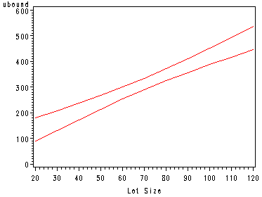
Example Confidence Bands including Fig. 2.6, p. 68-69.

proc reg data = ch1tab01 noprint;
  model y = x;
  output out = temp stdp=stdp p=p;
run;
data temp1;
  set temp;
  lbound = p - 2.258*stdp;
  ubound = p + 2.258*stdp;
run;
proc sort data = temp1;
  by x;
run;
 
symbol1 v=none i=join c=red;
symbol2 v=none i=join c=red;
proc gplot data = temp1;
  plot (ubound lbound)*x / overlay;
run;
quit;

Example of correlation coefficient and R-squared, p. 82.

proc corr data = ch1tab01;
 var x y;
run;
proc reg data = ch1tab01;
  model y =x;
run;
quit;

The CORR Procedure

2 Variables: x y

Simple Statistics

Variable N Mean Std Dev Sum Minimum Maximum Label

x 25 70.00000 28.72281 1750 20.00000 120.00000 Lot Size
y 25 312.28000 113.13764 7807 113.00000 546.00000 Work Hrs

Pearson Correlation Coefficients, N = 25
Prob > |r| under H0: Rho=0

x y

x 1.00000 0.90638
Lot Size <.0001

y 0.90638 1.00000
Work Hrs <.0001

The REG Procedure
Model: MODEL1
Dependent Variable: y Work Hrs

Analysis of Variance

Sum of Mean
Source DF Squares Square F Value Pr > F

Model 1 252378 252378 105.88 <.0001
Error 23 54825 2383.71562
Corrected Total 24 307203

Root MSE 48.82331 R-Square 0.8215
Dependent Mean 312.28000 Adj R-Sq 0.8138
Coeff Var 15.63447

Parameter Estimates

Parameter Standard
Variable Label DF Estimate Error t Value Pr > |t|

Intercept Intercept 1 62.36586 26.17743 2.38 0.0259
x Lot Size 1 3.57020 0.34697 10.29 <.0001