options nocenter nodate;
Inputting the Toluca Company data.
data ch1tab01;
  input x y;
  label x = 'Lot Size'
        y = 'Work Hrs';
cards;
   80  399
   30  121
   50  221
   90  376
   70  361
   60  224
  120  546
   80  352
  100  353
   50  157
   40  160
   70  252
   90  389
   20  113
  110  435
  100  420
   30  212
   50  268
   90  377
  110  421
   30  273
   90  468
   40  244
   80  342
   70  323
;
run;
Example of 90% Confidence Intervals for the regression parameter estimates, p. 154.
proc reg data = ch1tab01;
  model y = x/ clb;
run;
quit;
The REG Procedure
Model: MODEL1
Dependent Variable: y Work HrsAnalysis of Variance
Sum of Mean
Source DF Squares Square F Value Pr > F
Model 1 252378 252378 105.88 <.0001
Error 23 54825 2383.71562
Corrected Total 24 307203Root MSE 48.82331 R-Square 0.8215
Dependent Mean 312.28000 Adj R-Sq 0.8138
Coeff Var 15.63447Parameter Estimates
Parameter Standard
Variable Label DF Estimate Error t Value Pr > |t| 95% Confidence LimitsIntercept Intercept 1 62.36586 26.17743 2.38 0.0259 8.21371 116.51801
x Lot Size 1 3.57020 0.34697 10.29 <.0001 2.85244 4.28797Using the Working-Hotelling procedure to obtain a family of estimates and confidence intervals for mean working hours when X = 30, 65, 100 with a family confidence coefficient of 0.90, p. 156-157.data extra; input x y; cards; 30 . 65 . 100 . ; run; data temp; set ch1tab01 extra; run; ods listing close; ods output anova=out; proc reg data = temp; model y = x/ alpha=.1; output out=temp1 p=yhat stdi=stdi; run; quit; ods listing; data _null_; set out; if source = 'Error' then do; call symput ('mse', ms); call symput ('df', df ); end; run; %put &mse &df; /* To see the value of MSE and df in the log file. */ data temp2; set temp1; if y=.; syh = sqrt( (stdi)**2 - &mse ); f = finv(.90, 2, &df); w = sqrt( 2*f ); lower = yhat - w*syh; upper = yhat + w*syh; run; proc print data = temp2; var x yhat syh f w lower upper; run;Obs x yhat syh f w lower upper1 30 169.472 16.9697 2.54929 2.25800 131.154 207.790
2 65 294.429 9.9176 2.54929 2.25800 272.035 316.823
3 100 419.386 14.2723 2.54929 2.25800 387.159 451.613Using the Bonferroni procedure to obtain a family of estimates and confidence
intervals for mean working hours when X = 30, 65, 100 with a family confidence coefficient
of 0.90, p. 157.data extra; input x y; cards; 30 . 65 . 100 . ; run; data temp; set ch1tab01 extra; run; ods listing close; ods output anova=out; proc reg data = temp; model y = x/ alpha=.1; output out=temp1 p=yhat stdi=stdi; run; quit; ods listing; data _null_; set out; if source = 'Error' then do; call symput ('mse', ms); call symput ('df', df ); end; run; %put &mse &df; /* To see the value of MSE and df in the log file. */ data temp2; set temp1; if y=.; syh = sqrt( (stdi)**2 - &mse ); B = tinv( 1- (.1 /(2*3)), &df); lower = yhat - B*syh; upper = yhat + B*syh; run; proc print data = temp2; var x yhat syh B lower upper; run;Obs x yhat syh B lower upper1 30 169.472 16.9697 2.26373 131.057 207.887
2 65 294.429 9.9176 2.26373 271.978 316.880
3 100 419.386 14.2723 2.26373 387.077 451.695Simultaneous Prediction intervals for new observations, p. 158-159.
data extra; input x y; cards; 80 . 100 . ; run; data temp; set ch1tab01 extra; run; proc reg data = temp noprint; model y = x/ alpha=.1; output out=temp1 p=yhat stdi=spred; run; quit; data temp2; set temp1; if y=.; s = sqrt( 2*finv(.95, 2, 23) ); B = tinv( 1 - (.05/(2*2)), 23) ; lowers = yhat - s*spred; uppers = yhat + s*spred; lowerb = yhat - b*spred; upperb = yhat + b*spred; run; proc print data = temp2; var x yhat spred b lowerb upperb s lowers uppers; run;Obs x yhat spred B lowerb upperb s lowers uppersc1 80 347.982 49.9110 2.39788 228.302 467.662 2.61615 217.407 478.557
2 100 419.386 50.8666 2.39788 297.414 541.358 2.61615 286.311 552.461Inputting the Warehouse data, table 4.2, p. 161.
data ch4tab02; input x y; label x = 'Work' y = 'Labor'; cards; 20 114 196 921 115 560 50 245 122 575 100 475 33 138 154 727 80 375 147 670 182 828 160 762 ; run;Creating the interaction between X and Y, the X^2 and the predicted Y-hat values. The rest
of table 4.2, p. 161.data ch4tab02; set ch4tab02; xy = x*y; xsq = x**2; run; proc reg data = ch4tab02 noprint; model y = x /noint; output out= temp p=yhat r=e; run; proc print data = temp (obs = 5); run;Obs x y xy xsq yhat e1 20 114 2280 400 93.705 20.2945
2 196 921 180516 38416 918.314 2.6863
3 115 560 64400 13225 538.807 21.1935
4 50 245 12250 2500 234.264 10.7363
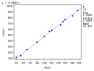
5 122 575 70150 14884 571.603 3.3966Fig. 4.1 and calculations on p. 162.
goptions reset = all; symbol v=dot h=.8 c=blue; proc reg data = temp; model y = x/ noint clb; plot y*x; run; quit;
The REG Procedure
Model: MODEL1
Dependent Variable: y LaborNOTE: No intercept in model. R-Square is redefined.
Analysis of Variance
Sum of Mean
Source DF Squares Square F Value Pr > FModel 1 4191980 4191980 18762.5 <.0001
Error 11 2457.65933 223.42358
Uncorrected Total 12 4194438Root MSE 14.94736 R-Square 0.9994
Dependent Mean 532.50000 Adj R-Sq 0.9994
Coeff Var 2.80702Parameter Estimates
Parameter Standard
Variable Label DF Estimate Error t Value Pr > |t| 95% Confidence Limitsx Work 1 4.68527 0.03421 136.98 <.0001 4.60999 4.76056
The Calibration example p. 168 was not reproduced.