
Table 5.1 on page 78, Table 5.2 on page 79 using data file
gpa.
proc glm data = gpa;
 class sex;
  model gpa1-gpa6 = sex highgpa /nouni ;
  repeated gpa 6 polynomial / summary;
run;
quit;
Repeated Measures Analysis of Variance

Manova Test Criteria and Exact F Statistics for the Hypothesis of no gpa Effect
                       H = Type III SSCP Matrix for gpa
                             E = Error SSCP Matrix
                            S=1    M=1.5    N=95.5
Statistic                        Value    F Value    Num DF    Den DF    Pr > F
Wilks' Lambda               0.89503663       4.53         5       193    0.0006
Pillai's Trace              0.10496337       4.53         5       193    0.0006
Hotelling-Lawley Trace      0.11727271       4.53         5       193    0.0006
Roy's Greatest Root         0.11727271       4.53         5       193    0.0006

Manova Test Criteria and Exact F Statistics for the Hypothesis of no gpa*SEX Effect
                       H = Type III SSCP Matrix for gpa*SEX
                               E = Error SSCP Matrix
                              S=1    M=1.5    N=95.5
Statistic                        Value    F Value    Num DF    Den DF    Pr > F
Wilks' Lambda               0.96457680       1.42         5       193    0.2196
Pillai's Trace              0.03542320       1.42         5       193    0.2196
Hotelling-Lawley Trace      0.03672408       1.42         5       193    0.2196
Roy's Greatest Root         0.03672408       1.42         5       193    0.2196

Manova Test Criteria and Exact F Statistics for the Hypothesis of no gpa*HIGHGPA Effect
                       H = Type III SSCP Matrix for gpa*HIGHGPA
                                 E = Error SSCP Matrix
                                S=1    M=1.5    N=95.5
Statistic                        Value    F Value    Num DF    Den DF    Pr > F
Wilks' Lambda               0.97806928       0.87         5       193    0.5053
Pillai's Trace              0.02193072       0.87         5       193    0.5053
Hotelling-Lawley Trace      0.02242246       0.87         5       193    0.5053
Roy's Greatest Root         0.02242246       0.87         5       193    0.5053
Tests of Hypotheses for Between Subjects Effects
Source                      DF     Type III SS     Mean Square    F Value    Pr > F
SEX                          1      7.22715867      7.22715867      18.37    <.0001
HIGHGPA                      1      3.60320801      3.60320801       9.16    0.0028
Error                      197     77.49355890      0.39336832
proc means data = gpa mean std N;
 class sex;
var gpa1 - gpa6;
run;
The MEANS Procedure
                  N
         SEX    Obs    Variable            Mean         Std Dev      N
--------------------------------------------------------------------------------------------------------
           1     95    GPA1           2.5547368       0.3137855     95
                       GPA2           2.6663158       0.3177750     95
                       GPA3           2.7421053       0.3630776     95
                       GPA4           2.8178947       0.3509801     95
                       GPA5           2.9147368       0.3587711     95
                       GPA6           3.0284211       0.3752058     95
           2    105    GPA1           2.6285714       0.3071940    105
                       GPA2           2.7600000       0.3476846    105
                       GPA3           2.8714286       0.3350414    105
                       GPA4           3.0085714       0.3354430    105
                       GPA5           3.1133333       0.3319716    105
                       GPA6           3.2295238       0.3538045    105
--------------------------------------------------------------------------------------------------------
Figure 5.3 on page 80 using data file gpachp5.
proc univariate data = gpachp5 noprint;
histogram gpa /normal vscale=count
               nohlabel cfill = grey midpoints=(1.75 to 4 by .25);
inset mean std n;
run;
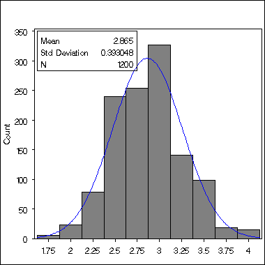
Table 5.3 on page 81 using data file
gpa4chp5. Notice that the results for Part 3 and Part 4 are a little
different from the book.
Part 1: Null model.
proc mixed data = gpachp5 covtest method = ml;
  model gpa =   /solution;
  random intercept /subject = student;
run;
The Mixed Procedure
                  Covariance Parameter Estimates
                                     Standard         Z
Cov Parm      Subject    Estimate       Error     Value        Pr Z
Intercept     STUDENT     0.05677    0.007339      7.73      <.0001
Residual                  0.09759    0.004364     22.36      <.0001

           Fit Statistics
-2 Log Likelihood               913.5
AIC (smaller is better)         919.5
AICC (smaller is better)        919.5
BIC (smaller is better)         929.4

                   Solution for Fixed Effects
                         Standard
Effect       Estimate       Error      DF    t Value    Pr > |t|
Intercept      2.8650     0.01911     199     149.93      <.0001
Part 2: With additional variable time which is created as
follow.
proc mixed data = gpachp5 covtest method = ml;
  model gpa = time  /solution;
  random intercept /subject = student;
run;
The Mixed Procedure
                  Covariance Parameter Estimates
                                     Standard         Z
Cov Parm      Subject    Estimate       Error     Value        Pr Z
Intercept     STUDENT     0.06336    0.007316      8.66      <.0001
Residual                  0.05803    0.002595     22.36      <.0001

           Fit Statistics
-2 Log Likelihood               393.6
AIC (smaller is better)         401.6
AICC (smaller is better)        401.7
BIC (smaller is better)         414.8

                   Solution for Fixed Effects
                         Standard
Effect       Estimate       Error      DF    t Value    Pr > |t|
Intercept      2.5992     0.02165     199     120.05      <.0001
TIME           0.1063    0.004072     999      26.11      <.0001
Part 3: The variable job is added.
proc mixed data = gpachp5 covtest method = ml;
  model gpa = time job /solution;
  random intercept /subject = student type = un;
run;
                  Covariance Parameter Estimates
                                    Standard         Z
Cov Parm     Subject    Estimate       Error     Value        Pr Z
UN(1,1)      STUDENT     0.05336    0.006371      8.38      <.0001
Residual                 0.05561    0.002494     22.30      <.0001

           Fit Statistics
-2 Log Likelihood               320.3
AIC (smaller is better)         330.3
AICC (smaller is better)        330.3
BIC (smaller is better)         346.8

                   Solution for Fixed Effects
                         Standard
Effect       Estimate       Error      DF    t Value    Pr > |t|
Intercept      2.9458     0.04446     199      66.26      <.0001
TIME           0.1032    0.004002     998      25.78      <.0001
JOB           -0.1609     0.01836     998      -8.76      <.0001
Part 4: The variable highgpa and sex are added to the
model and sex should be treated as categorical variable.
proc mixed data = gpachp5 covtest method = ml;
  class sex;
  model gpa = time job highgpa sex /solution;
  random intercept /subject = student type=un;
run;
Covariance Parameter Estimates
                                    Standard         Z
Cov Parm     Subject    Estimate       Error     Value        Pr Z
UN(1,1)      STUDENT     0.04576    0.005606      8.16      <.0001
Residual                 0.05562    0.002495     22.29      <.0001
Fit Statistics
-2 Log Likelihood               294.5
AIC (smaller is better)         308.5
AICC (smaller is better)        308.6
BIC (smaller is better)         331.6
Null Model Likelihood Ratio Test
DF Chi-Square Pr > ChiSq
1 333.27 <.0001
Solution for Fixed Effects
             student                Standard
Effect       gender     Estimate       Error      DF    t Value    Pr > |t|
Intercept                 2.7618     0.09548     197      28.93      <.0001
TIME                      0.1031    0.004002     998      25.77      <.0001
JOB                      -0.1618     0.01830     998      -8.84      <.0001
HIGHGPA                  0.08584     0.02798     998       3.07      0.0022
SEX          1           -0.1484     0.03331     998      -4.45      <.0001
SEX          2                 0           .       .        .         .
Table 5.4 on page 83.
Part 1: The variable time is included as a random effect.
proc mixed data = gpachp5 covtest method = ml;
  class sex;
  model gpa = time job highgpa sex /solution;
  random intercept time/subject = student type=un;
run;
                  Covariance Parameter Estimates

                                    Standard         Z
Cov Parm     Subject    Estimate       Error     Value        Pr Z

UN(1,1)      STUDENT     0.03897    0.006221      6.26      <.0001
UN(2,1)      STUDENT    -0.00256    0.001558     -1.65      0.0999
UN(2,2)      STUDENT    0.003912    0.000646      6.06      <.0001
Residual                 0.04176    0.002099     19.89      <.0001


           Fit Statistics

-2 Log Likelihood               180.2
AIC (smaller is better)         198.2
AICC (smaller is better)        198.4
BIC (smaller is better)         227.9


  Null Model Likelihood Ratio Test

    DF    Chi-Square      Pr > ChiSq

     3        447.61          <.0001


                        Solution for Fixed Effects

             student                Standard
Effect       gender     Estimate       Error      DF    t Value    Pr > |t|

Intercept                 2.6440     0.08999     197      29.38      <.0001
TIME                      0.1040    0.005622     199      18.49      <.0001
JOB                      -0.1196     0.01746     799      -6.85      <.0001
HIGHGPA                  0.08984     0.02647     799       3.39      0.0007
SEX          1           -0.1168     0.03153     799      -3.70      0.0002
SEX          2                 0           .       .        .         .
Part 2: Cross level interaction of variable time and sex
is included. We first created the interaction term.
proc mixed data = gpachp5 covtest method = ml;
  class sex;
  model gpa = time job highgpa sex time*sex/solution;
  random intercept time /subject = student type=un;
run;
                  Covariance Parameter Estimates

                                    Standard         Z
Cov Parm     Subject    Estimate       Error     Value        Pr Z

UN(1,1)      STUDENT     0.03855    0.006149      6.27      <.0001
UN(2,1)      STUDENT    -0.00227    0.001506     -1.51      0.1310
UN(2,2)      STUDENT    0.003690    0.000624      5.91      <.0001
Residual                 0.04178    0.002101     19.89      <.0001


           Fit Statistics

-2 Log Likelihood               173.2
AIC (smaller is better)         193.2
AICC (smaller is better)        193.4
BIC (smaller is better)         226.2


  Null Model Likelihood Ratio Test

    DF    Chi-Square      Pr > ChiSq

     3        446.52          <.0001


                        Solution for Fixed Effects

             student                Standard
Effect       gender     Estimate       Error      DF    t Value    Pr > |t|

Intercept                 2.6273     0.09018     197      29.14      <.0001
TIME                      0.1180    0.007614     198      15.49      <.0001
JOB                      -0.1206     0.01743     799      -6.92      <.0001
HIGHGPA                  0.08981     0.02646     799       3.39      0.0007
SEX          1          -0.07680     0.03490     799      -2.20      0.0281
SEX          2                 0           .       .        .         .
TIME*SEX     1          -0.02947     0.01104     799      -2.67      0.0077
TIME*SEX     2                 0           .       .        .         .
Figure 5.4 on page 84.
proc mixed data = gpachp5 method = ml;
  class sex;
  model gpa = time job highgpa sex time*sex/solution ;
  random intercept time /subject = student type=un;
run;
data fig54;
  set gpachp5;
  pred = 2.63 + 0.12*time -0.07682*(sex=1) - 0.02947*time*(sex=1);
run;

symbol1 i = join r=2 v=circle;
axis1 order = (2.5 to 3.3 by .1) minor = none label=(a= 90 "Predicted GPA");
axis2 order = (0 to 6 by 1) minor = none label=("Time");
proc gplot data = fig54;
  plot pred*time = sex /vaxis = axis1 haxis = axis2;
run;
quit;
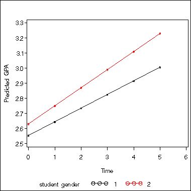
Table 5.5 on page 85.
data table55;
  set gpachp5;
  t1 = time;
  t2 = time - 5;
  t3 = time - 2.5;
run;
Part 1: First occasion = 0.
proc mixed data = table55 covtest method = ml;
  class sex;
  model gpa = t1 job highgpa sex /solution ;
  random intercept t1/subject = student type=un;
run;
                  Covariance Parameter Estimates

                                    Standard         Z
Cov Parm     Subject    Estimate       Error     Value        Pr Z

UN(1,1)      STUDENT     0.03897    0.006221      6.26      <.0001
UN(2,1)      STUDENT    -0.00256    0.001558     -1.65      0.0999
UN(2,2)      STUDENT    0.003912    0.000646      6.06      <.0001
Residual                 0.04176    0.002099     19.89      <.0001


           Fit Statistics

-2 Log Likelihood               180.2
AIC (smaller is better)         198.2
AICC (smaller is better)        198.4
BIC (smaller is better)         227.9


  Null Model Likelihood Ratio Test

    DF    Chi-Square      Pr > ChiSq

     3        447.61          <.0001


                        Solution for Fixed Effects

             student                Standard
Effect       gender     Estimate       Error      DF    t Value    Pr > |t|

Intercept                 2.6440     0.08999     197      29.38      <.0001
t1                        0.1040    0.005622     199      18.49      <.0001
JOB                      -0.1196     0.01746     799      -6.85      <.0001
HIGHGPA                  0.08984     0.02647     799       3.39      0.0007
SEX          1           -0.1168     0.03153     799      -3.70      0.0002
SEX          2                 0           .       .        .         .
Part 2: The variable time has been recoded as -5, …,-1, 0, …with the
last occasion coded as zero. This is variable t2.
proc mixed data = table55 covtest method = ml;
  class sex;
  model gpa = t2 job highgpa sex /solution ;
  random intercept t2/subject = student type=un;
run;
                  Covariance Parameter Estimates

                                    Standard         Z
Cov Parm     Subject    Estimate       Error     Value        Pr Z

UN(1,1)      STUDENT      0.1111     0.01373      8.09      <.0001
UN(2,1)      STUDENT     0.01700    0.002676      6.35      <.0001
UN(2,2)      STUDENT    0.003912    0.000646      6.06      <.0001
Residual                 0.04176    0.002099     19.89      <.0001


           Fit Statistics

-2 Log Likelihood               180.2
AIC (smaller is better)         198.2
AICC (smaller is better)        198.4
BIC (smaller is better)         227.9


  Null Model Likelihood Ratio Test

    DF    Chi-Square      Pr > ChiSq

     3        447.61          <.0001


                        Solution for Fixed Effects

             student                Standard
Effect       gender     Estimate       Error      DF    t Value    Pr > |t|

Intercept                 3.1639     0.09127     197      34.67      <.0001
t2                        0.1040    0.005622     199      18.49      <.0001
JOB                      -0.1196     0.01746     799      -6.85      <.0001
HIGHGPA                  0.08984     0.02647     799       3.39      0.0007
SEX          1           -0.1168     0.03153     799      -3.70      0.0002
SEX          2                 0           .       .        .         .
Part 3: The variable time is recoded centered around its mean and
is included as a fixed effect. This is variable t3.
proc mixed data = table55 covtest method = ml;
  class sex;
  model gpa = t3 job highgpa sex /solution ;
  random intercept t3/subject = student type=un;
run;
                  Covariance Parameter Estimates

                                    Standard         Z
Cov Parm     Subject    Estimate       Error     Value        Pr Z

UN(1,1)      STUDENT     0.05060    0.005885      8.60      <.0001
UN(2,1)      STUDENT    0.007217    0.001480      4.88      <.0001
UN(2,2)      STUDENT    0.003912    0.000646      6.06      <.0001
Residual                 0.04176    0.002099     19.89      <.0001


           Fit Statistics

-2 Log Likelihood               180.2
AIC (smaller is better)         198.2
AICC (smaller is better)        198.4
BIC (smaller is better)         227.9


  Null Model Likelihood Ratio Test

    DF    Chi-Square      Pr > ChiSq

     3        447.61          <.0001


                        Solution for Fixed Effects

             student                Standard
Effect       gender     Estimate       Error      DF    t Value    Pr > |t|

Intercept                 2.9040     0.08953     197      32.44      <.0001
t3                        0.1040    0.005622     199      18.49      <.0001
JOB                      -0.1196     0.01746     799      -6.85      <.0001
HIGHGPA                  0.08984     0.02647     799       3.39      0.0007
SEX          1           -0.1168     0.03153     799      -3.70      0.0002
SEX          2                 0           .       .        .         .
Table 5.6 using data file vocagrwt.
proc freq data = vocagrwt ;
  tables age /nopercent nocum ;
run;
The FREQ Procedure
AGE    Frequency
----------------
 12          22
 14           5
 16          22
 18          11
 20          22
 22          11
 24          22
 26          11
Table 5.7 on page 89. We will create all the variables needed for this
table in the following data step.
data voca;
  set in.vocagrwt;
  sdummy = study - .5;
  agec = age - 18.889;
  agec2 = agec*agec;
run;
Part 1: Intercept only model.
proc mixed data = voca covtest method = ml;
  model vocab = sdummy /solution;
  random intercept /subject = child type = un;
run;
                  Covariance Parameter Estimates
                                    Standard         Z
Cov Parm     Subject    Estimate       Error     Value        Pr Z
UN(1,1)      CHILD       2400.41     2147.95      1.12      0.1319
Residual                   31076     4201.58      7.40      <.0001

           Fit Statistics
-2 Log Likelihood              1668.9
AIC (smaller is better)        1676.9
AICC (smaller is better)       1677.2
BIC (smaller is better)        1681.3

                   Solution for Fixed Effects
                         Standard
Effect       Estimate       Error      DF    t Value    Pr > |t|
Intercept      132.07     19.5083      20       6.77      <.0001
sdummy        -110.91     39.0165     104      -2.84      0.005
Part 2: The variable age is grand mean centered and is included as a
fixed effect. This is variable agec.
proc mixed data = voca covtest method = ml;
  model vocab = sdummy agec/solution;
  random intercept /subject = child type = un;
run;
                  Covariance Parameter Estimates
                                    Standard         Z
Cov Parm     Subject    Estimate       Error     Value        Pr Z
UN(1,1)      CHILD       4882.74     1937.08      2.52      0.0059
Residual                   10377     1421.19      7.30      <.0001
           Fit Statistics
-2 Log Likelihood              1550.9
AIC (smaller is better)        1560.9
AICC (smaller is better)       1561.4
BIC (smaller is better)        1566.4

                   Solution for Fixed Effects
                         Standard
Effect       Estimate       Error      DF    t Value    Pr > |t|
Intercept      137.78     17.6864      20       7.79      <.0001
sdummy       -69.7926     35.4737     103      -1.97      0.0518
agec          29.5553      2.0138     103      14.68      <.0001
Part 3: The squared term of agec is included as a fixed effect.
proc mixed data = voca covtest method = ml;
  model vocab = sdummy agec agec2/solution;
  random intercept /subject = child type = un;
run;
                  Covariance Parameter Estimates
                                    Standard         Z
Cov Parm     Subject    Estimate       Error     Value        Pr Z
UN(1,1)      CHILD       5166.25     1902.71      2.72      0.0033
Residual                 7721.24     1060.15      7.28      <.0001
           Fit Statistics
-2 Log Likelihood              1519.5
AIC (smaller is better)        1531.5
AICC (smaller is better)       1532.2
BIC (smaller is better)        1538.0

                   Solution for Fixed Effects
                         Standard
Effect       Estimate       Error      DF    t Value    Pr > |t|
Intercept     84.7951     19.4698      20       4.36      0.0003
sdummy       -68.2509     34.8592     102      -1.96      0.0530
agec          30.6225      1.7460     102      17.54      <.0001
agec2          2.5573      0.4227     102       6.05      <.0001
Part 4: Centered variable agec is included as a random effect.
proc mixed data = voca covtest method = ml;
  model vocab = sdummy agec agec2/solution;
  random intercept agec/subject = child type = un;
run;
                  Covariance Parameter Estimates
                                    Standard         Z
Cov Parm     Subject    Estimate       Error     Value        Pr Z
UN(1,1)      CHILD       6453.59     1999.97      3.23      0.0006
UN(2,1)      CHILD       1267.44      384.64      3.30      0.0010
UN(2,2)      CHILD        240.39     74.6448      3.22      0.0006
Residual                  941.02      135.58      6.94      <.0001

           Fit Statistics
-2 Log Likelihood              1290.0
AIC (smaller is better)        1306.0
AICC (smaller is better)       1307.2
BIC (smaller is better)        1314.7

                   Solution for Fixed Effects
                         Standard
Effect       Estimate       Error      DF    t Value    Pr > |t|
Intercept     88.0805     17.6336      20       5.00      <.0001
sdummy        -3.6132      5.3738      81      -0.67      0.5033
agec          28.1058      3.3675      21       8.35      <.0001
agec2          2.1792      0.1518      81      14.36      <.0001
Table 5.8 on page 91.
Part 1: Intercept only model.
proc mixed data = voca covtest method = ml;
  model vocab = sdummy/solution;
  random intercept /subject = child type = un;
run;
                  Covariance Parameter Estimates
                                    Standard         Z
Cov Parm     Subject    Estimate       Error     Value        Pr Z
UN(1,1)      CHILD       2400.41     2147.95      1.12      0.1319
Residual                   31076     4201.58      7.40      <.0001

           Fit Statistics
-2 Log Likelihood              1668.9
AIC (smaller is better)        1676.9
AICC (smaller is better)       1677.2
BIC (smaller is better)        1681.3

                   Solution for Fixed Effects
                         Standard
Effect       Estimate       Error      DF    t Value    Pr > |t|
Intercept      132.07     19.5083      20       6.77      <.0001
sdummy        -110.91     39.0165     104      -2.84      0.0054
Part 2: The variable age is centered on 12 months and is included
as a fixed effect.
proc mixed data = voca covtest method = ml;
  model vocab = sdummy age12/solution;
  random intercept /subject = child type = un;
run;
                  Covariance Parameter Estimates
                                    Standard         Z
Cov Parm     Subject    Estimate       Error     Value        Pr Z
UN(1,1)      CHILD       4882.74     1937.08      2.52      0.0059
Residual                   10377     1421.19      7.30      <.0001

           Fit Statistics
-2 Log Likelihood              1550.9
AIC (smaller is better)        1560.9
AICC (smaller is better)       1561.4
BIC (smaller is better)        1566.4

                   Solution for Fixed Effects
                         Standard
Effect       Estimate       Error      DF    t Value    Pr > |t|
Intercept    -65.8220     22.2324      20      -2.96      0.0077
sdummy       -69.7926     35.4737     103      -1.97      0.0518
AGE12         29.5553      2.0138     103      14.68      <.0001
Part 3: The variable age12sq is included as a fixed effect.
proc mixed data = voca covtest method = ml;
  model vocab = sdummy age12 age12sq/solution;
  random intercept /subject = child type = un;
run;
                  Covariance Parameter Estimates
                                    Standard         Z
Cov Parm     Subject    Estimate       Error     Value        Pr Z
UN(1,1)      CHILD       5166.25     1902.71      2.72      0.0033
Residual                 7721.24     1060.15      7.28      <.0001

           Fit Statistics
-2 Log Likelihood              1519.5
AIC (smaller is better)        1531.5
AICC (smaller is better)       1532.2
BIC (smaller is better)        1538.0

                   Solution for Fixed Effects
                         Standard
Effect       Estimate       Error      DF    t Value    Pr > |t|
Intercept     -4.7972     23.2299      20      -0.21      0.8385
sdummy       -68.2509     34.8592     102      -1.96      0.0530
AGE12         -4.6122      5.9106     102      -0.78      0.4370
AGE12SQ        2.5573      0.4227     102       6.05      <.0001
Part 4: The variable age12 is a random effect.
proc mixed data = voca covtest method = ml;
  model vocab = sdummy age12 age12sq/solution;
  random intercept age12 /subject = child type = un;
run;
                  Covariance Parameter Estimates
                                    Standard         Z
Cov Parm     Subject    Estimate       Error     Value        Pr Z
UN(1,1)      CHILD        399.28      271.79      1.47      0.0709
UN(2,1)      CHILD       -388.63      136.43     -2.85      0.0044
UN(2,2)      CHILD        240.41     74.6570      3.22      0.0006
Residual                  941.01      135.57      6.94      <.0001
           Fit Statistics
-2 Log Likelihood              1290.0
AIC (smaller is better)        1306.0
AICC (smaller is better)       1307.2
BIC (smaller is better)        1314.7

                   Solution for Fixed Effects
                         Standard
Effect       Estimate       Error      DF    t Value    Pr > |t|
Intercept     -2.1174      7.3727      20      -0.29      0.7769
sdummy        -3.6130      5.3738      81      -0.67      0.5033
AGE12         -1.9198      3.9040      21      -0.49      0.6280
AGE12SQ        2.1792      0.1518      81      14.36      <.0001
Table 5.9 on page 92 is created using HLM. We omit it here.
Table 5.10 on page 101 using data file gpa4chp5.
Part 1: The variable time is a fixed effect. We have built the
model at the beginning of this chapter. We will use it here.
proc mixed data = gpachp5 covtest method = ml;
  model gpa = time job highgpa sex /solution;
  random intercept /subject = student type=un;
run;
                  Covariance Parameter Estimates
                                    Standard         Z
Cov Parm     Subject    Estimate       Error     Value        Pr Z
UN(1,1)      STUDENT     0.04576    0.005606      8.16      <.0001
Residual                 0.05562    0.002495     22.29      <.0001

           Fit Statistics
-2 Log Likelihood               294.5
AIC (smaller is better)         308.5
AICC (smaller is better)        308.6
BIC (smaller is better)         331.6

                   Solution for Fixed Effects
                         Standard
Effect       Estimate       Error      DF    t Value    Pr > |t|
Intercept      2.4651      0.1113     197      22.15      <.0001
TIME           0.1031    0.004002     998      25.77      <.0001
JOB           -0.1618     0.01830     998      -8.84      <.0001
HIGHGPA       0.08584     0.02798     998       3.07      0.0022
SEX            0.1484     0.03331     998       4.45      <.0001
Part 2: The variable time is included as random effect.
proc mixed data = gpachp5 covest method = ml;
  model gpa = time job highgpa sex  /solution;
  random intercept time /subject = student type=un;
run;
                  Covariance Parameter Estimates
                                    Standard         Z
Cov Parm     Subject    Estimate       Error     Value        Pr Z
UN(1,1)      STUDENT     0.03897    0.006221      6.26      <.0001
UN(2,1)      STUDENT    -0.00256    0.001558     -1.65      0.0999
UN(2,2)      STUDENT    0.003912    0.000646      6.06      <.0001
Residual                 0.04176    0.002099     19.89      <.0001

           Fit Statistics
-2 Log Likelihood               180.2
AIC (smaller is better)         198.2
AICC (smaller is better)        198.4
BIC (smaller is better)         227.9

                   Solution for Fixed Effects
                         Standard
Effect       Estimate       Error      DF    t Value    Pr > |t|
Intercept      2.4105      0.1051     197      22.94      <.0001
TIME           0.1040    0.005622     199      18.49      <.0001
JOB           -0.1196     0.01746     799      -6.85      <.0001
HIGHGPA       0.08984     0.02647     799       3.39      0.0007
SEX            0.1168     0.03153     799       3.70      0.0002
Part 3: The variable time is a fixed effect, MANOVA.
proc mixed data = gpachp5 dfbw covtest method = ml noitprint;
  class occas;
  model gpa = time job highgpa sex  / solution;
  repeated occas / subject=student type= un ;
run;
The Mixed Procedure
                 Covariance Parameter Estimates
                                   Standard         Z
Cov Parm    Subject    Estimate       Error     Value        Pr Z
UN(1,1)     STUDENT     0.09208    0.009261      9.94      <.0001
UN(2,1)     STUDENT     0.03072    0.007211      4.26      <.0001
UN(2,2)     STUDENT      0.1020     0.01027      9.93      <.0001
UN(3,1)     STUDENT     0.02018    0.007249      2.78      0.0054
UN(3,2)     STUDENT     0.03878    0.008013      4.84      <.0001
UN(3,3)     STUDENT      0.1094     0.01098      9.96      <.0001
UN(4,1)     STUDENT     0.01380    0.007127      1.94      0.0528
UN(4,2)     STUDENT     0.04121    0.008046      5.12      <.0001
UN(4,3)     STUDENT     0.06847    0.009147      7.49      <.0001
UN(4,4)     STUDENT      0.1078     0.01090      9.89      <.0001
UN(5,1)     STUDENT     0.01571    0.007035      2.23      0.0256
UN(5,2)     STUDENT     0.04632    0.008063      5.74      <.0001
UN(5,3)     STUDENT     0.07114    0.009208      7.73      <.0001
UN(5,4)     STUDENT     0.08566    0.009831      8.71      <.0001
UN(5,5)     STUDENT      0.1042     0.01062      9.81      <.0001
UN(6,1)     STUDENT     0.01774    0.007470      2.38      0.0175
UN(6,2)     STUDENT     0.04027    0.008311      4.85      <.0001
UN(6,3)     STUDENT     0.07210    0.009591      7.52      <.0001
UN(6,4)     STUDENT     0.08961     0.01039      8.63      <.0001
UN(6,5)     STUDENT     0.09486     0.01055      8.99      <.0001
UN(6,6)     STUDENT      0.1170     0.01194      9.80      <.0001

           Fit Statistics
-2 Log Likelihood                -4.1
AIC (smaller is better)          47.9
AICC (smaller is better)         49.1
BIC (smaller is better)         133.7

                   Solution for Fixed Effects
                         Standard
Effect       Estimate       Error      DF    t Value    Pr > |t|
Intercept      2.3640      0.1025     197      23.06      <.0001
TIME           0.1047    0.004835     197      21.65      <.0001
JOB          -0.09300     0.01429     197      -6.51      <.0001
HIGHGPA       0.08442     0.02650     197       3.19      0.0017
SEX            0.1193     0.03156     197       3.78      0.0002