
The aim of this seminar is to
help you increase your skills in analyzing repeated
measures data using SAS. The seminar will describe conventional
ways to analyze repeated measures using SAS PROC GLM and describe
the assumptions and limitations of such conventional methods. Then we will
explore the use of SAS PROC MIXED for repeated measures analyses.
SAS Program for seminar.
There are a number of situations that can arise when the analysis includes
between groups effects as well as within subject effects. We
start by showing 4 example analyses using measurements of depression over 3 time
points broken down by 2 treatment groups. In the first
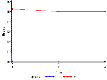
example we see that the two groups differ in
depression but neither group changes over time.
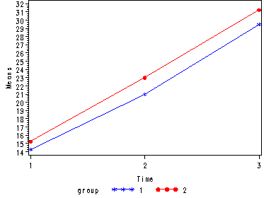
In the second example the two groups grow in depression but at the same rate
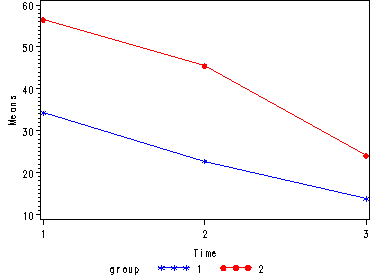
over time. In the third example, the two groups
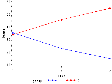
start off being quite different in depression but end up being rather close in depression. The fourth example shows the groups starting off at the same
level of depression, and one group group increases over time
whereas the other group decreases over time.
Note that in the interest of making learning the concepts easier we have taken the
liberty of using only a very small portion of the voluminous
output that SAS provides and we have inserted the graphs as needed to facilitate
understanding the concepts. The rather long code needed to actually create
the graphs in SAS has been included at the very end after all the output and
explanation.
Demo Analysis #1
The between groups test indicates that there the variable group is significant, consequently in the graph we see that
the lines for the two groups are rather far apart. The within subject test indicate that there is not a
significant time effect, in other words, the groups do not change
in depression over
time. In the graph we see that the groups have lines that are flat, i.e. the
slopes of the lines are approximately equal to zero.
Also, since the lines are parallel, we are not surprised that the
interaction between time and group is not significant.
<Abbreviated output from proc glm>


Tests of Hypotheses for Between Subjects Effects

Source                     DF    Type III SS    Mean Square   F Value   Pr > F
GROUP                       1    155.0416667    155.0416667   3721.00   <.0001
Error                       6      0.2500000      0.0416667

Univariate Tests of Hypotheses for Within Subject Effects

Source                     DF    Type III SS    Mean Square   F Value   Pr > F
time                        2     0.08333333     0.04166667      1.00   0.3966
time*GROUP                  2     0.08333333     0.04166667      1.00   0.3966
Error(time)                12     0.50000000     0.04166667
Demo Analysis #2
The between groups test indicates that there the variable group is not significant, consequently in the graph we see that
the lines for the two groups are rather close together. The within subject test indicate that there is a
significant time effect, in other words, the groups do change
in depression over time. In the graph we see that the groups have lines that increase over time.
Again, the lines are parallel consistent with the finding
that the interaction is not significant.
<Abbreviated output from proc glm>
Tests of Hypotheses for Between Subjects Effects

Source                     DF    Type III SS    Mean Square   F Value   Pr > F
GROUP                       1     15.0416667     15.0416667      0.84   0.3957
Error                       6    107.9166667     17.9861111

Univariate Tests of Hypotheses for Within Subject Effects

Source                     DF    Type III SS    Mean Square   F Value   Pr > F
time                        2    978.2500000    489.1250000     53.68   <.0001
time*GROUP                  2      1.0833333      0.5416667      0.06   0.9426
Error(time)                12    109.3333333      9.1111111
Demo Analysis #3
The between groups test indicates that there the variable group is significant, consequently in the graph we see that
the lines for the two groups are rather far apart. The within subject test indicate that there is a
significant time effect, in other words, the groups do change over time,
both groups are getting less depressed over time.
Moreover, the interaction of time and group is significant which means that the
groups are changing over time but are changing in different ways, which means that in the graph the lines will
not be parallel. In the graph
we see that the groups have non-parallel lines that decrease over time and are getting
progressively closer together over time.
Tests of Hypotheses for Between Subjects Effects

Source                     DF    Type III SS    Mean Square   F Value   Pr > F
GROUP                       1    2035.041667    2035.041667    343.15   <.0001
Error                       6      35.583333       5.930556

Univariate Tests of Hypotheses for Within Subject Effects

Source                     DF    Type III SS    Mean Square   F Value   Pr > F
time                        2    2830.333333    1415.166667    553.76   <.0001
time*GROUP                  2     200.333333     100.166667     39.20   <.0001
Error(time)                12      30.666667       2.555556
Demo Analysis #4
The within subject test indicate that the interaction of time and group is significant. The
main effect of time is not significant. However, the significant interaction indicates that
the groups are changing over time and they are changing in
different ways, in other words, in the graph the lines of the groups will not be parallel.
The between groups test indicates that there the variable group is
significant. In the graph for this particular case we see that one group is
increasing in depression over time and the other group is decreasing
in depression over time.
Tests of Hypotheses for Between Subjects Effects

Source                     DF    Type III SS    Mean Square   F Value   Pr > F
GROUP                       1    2542.041667    2542.041667    628.96   <.0001
Error                       6      24.250000       4.041667

Univariate Tests of Hypotheses for Within Subject Effects

Source                     DF    Type III SS    Mean Square   F Value   Pr > F
time                        2       1.000000       0.500000      0.08   0.9246
time*GROUP                  2    1736.333333     868.166667    137.08   <.0001
Error(time)                12      76.000000       6.333333
Creating Graphs of the Means for Demo Analysis #4
The SAS code for creating the graph for demo=4.
/* We use the out option in the lsmeans statement to create the data set means. */
proc glm data=demo4;
  class group;
  model time1 time2 time3 = group;
  repeated time 3 ;
  lsmeans group / out=means;
run;
quit;

/*We want to look at the means to make sure we created the correct dataset.*/
proc print data=means;
run;

/* For a better understanding of all the gplot options used here please
visit our webpage on using proc gplot.*/

goptions reset=all;
symbol1 c=blue v=star h=.8 i=j;
symbol2 c=red v=dot h=.8 i=j;
axis1 label=(a=90 'Means');
axis2 label=('Time') value=('1' '2' '3');
proc gplot data=means;
  plot lsmean*_name_=group/ vaxis=axis1 haxis=axis2;
run;
quit;
Exercise data examples
The data consists of people who were randomly assigned to two different diets: low-fat and not low-fat
and three different types of exercise: at rest, walking leisurely and running. Their pulse rate was measured
at three different time points during their assigned exercise: at 1 minute, 15 minutes and 30 minutes.
data exercise;
  input id exertype diet time1 time2 time3;
cards;
1     1         1       85       85       88
2     1         1       90       92       93
3     1         1       97       97       94
4     1         1       80       82       83
5     1         1       91       92       91
6     1         2       83       83       84
7     1         2       87       88       90
8     1         2       92       94       95
9     1         2       97       99       96
10    1         2      100       97      100
11    2         1       86       86       84
12    2         1       93      103      104
13    2         1       90       92       93
14    2         1       95       96      100
15    2         1       89       96       95
16    2         2       84       86       89
17    2         2      103      109       90
18    2         2       92       96      101
19    2         2       97       98      100
20    2         2      102      104      103
21    3         1       93       98      110
22    3         1       98      104      112
23    3         1       98      105       99
24    3         1       87      132      120
25    3         1       94      110      116
26    3         2       95      126      143
27    3         2      100      126      140
28    3         2      103      124      140
29    3         2       94      135      130
30    3         2       99      111      150
;
run;
Exercise example, model 1 (time and diet)
Let us first consider the model including diet as the group variable.
The graph below suggests that the pulse rate is growing over time. The
pulse rates may vary for the 2 diets and it is possible that the pulse rate is
growing faster for the “red” diet than the “blue” diet.
proc glm data=exercise;
  class diet;
  model time1 time2 time3 = diet;
  repeated time 3 / printe;
run;
quit;
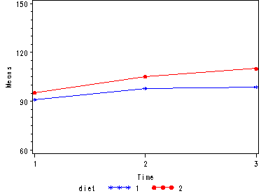
Looking at the results from the manova test
the effect of time is significant but the interaction of
time and diet is not significant. The between subject test of the
effect of
diet is also not significant. Consequently, in the graph we have lines
that are not flat, in fact, they are actually increasing over time, which was
expected since the effect of time was significant. Furthermore, the lines are
approximately parallel which was anticipated since the interaction was not
significant.
                            Sphericity Tests

                                   Mauchly's
Variables                    DF    Criterion    Chi-Square    Pr > ChiSq

Transformed Variates          2    0.4531199     21.373158        <.0001
Orthogonal Components         2     0.673336     10.678793        0.0048
Manova Test Criteria and Exact F Statistics for the Hypothesis of no time Effect
                       H = Type III SSCP Matrix for time
                             E = Error SSCP Matrix

                              S=1    M=0    N=12.5

Statistic                        Value    F Value    Num DF    Den DF    Pr > F
Wilks' Lambda               0.64349965       7.48         2        27    0.0026
Pillai's Trace              0.35650035       7.48         2        27    0.0026
Hotelling-Lawley Trace      0.55400240       7.48         2        27    0.0026
Roy's Greatest Root         0.55400240       7.48         2        27    0.0026


                  Manova Test Criteria and Exact F Statistics
                   for the Hypothesis of no time*DIET Effect
                     H = Type III SSCP Matrix for time*DIET
                             E = Error SSCP Matrix

                              S=1    M=0    N=12.5

Statistic                        Value    F Value    Num DF    Den DF    Pr > F
Wilks' Lambda               0.94402156       0.80         2        27    0.4595
Pillai's Trace              0.05597844       0.80         2        27    0.4595
Hotelling-Lawley Trace      0.05929784       0.80         2        27    0.4595
Roy's Greatest Root         0.05929784       0.80         2        27    0.4595

Tests of Hypotheses for Between Subjects Effects

Source                     DF    Type III SS    Mean Square   F Value   Pr > F
DIET                        1     1261.87778     1261.87778      3.15   0.0869
Error                      28    11227.02222      400.96508
Repeated Measures Analysis of Variance
Univariate Tests of Hypotheses for Within Subject Effects

Source                     DF    Type III SS    Mean Square   F Value   Pr > F
time                        2    2066.600000    1033.300000     11.81   <.0001
time*diet                   2     192.822222      96.411111      1.10   0.3394
Error(time)                56    4900.577778      87.510317

                          Adj Pr > F
Source                  G - G     H - F
time                   0.0003    0.0002
time*diet              0.3264    0.3303
Error(time)

Greenhouse-Geisser Epsilon    0.7538
Huynh-Feldt Epsilon           0.8158
Exercise example, model
2 (time and exercise type)
Next, let us consider the model including exertype as the group variable.
proc glm data=exercise;
  class exertype;
  model time1 time2 time3 = exertype;
  repeated time 3 ;
run;
quit;
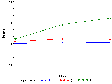
The interaction of time and exertype is significant as is the
effect of time. The between subject test of the effect of exertype is
also significant. Consequently, in the graph we have lines that are not parallel which we expected
since the interaction was significant. Furthermore, we see that some of the lines that are rather far
apart and at least one line is not horizontal which was anticipated since exertype and time
were both significant. The output for this analysis is
omitted.
Here is the code for the graph.
proc glm data=exercise;
  class exertype;
  model time1 time2 time3 = exertype;
  repeated time 3 ;
  lsmeans exertype / out=means;
run;
quit;
proc print data=means;
run;

goptions reset=all;
symbol1 c=blue v=star h=.8 i=j;
symbol2 c=red v=dot h=.8 i=j;
symbol3 c=green v=square h=.8 i=j;
axis1 order=(60 to 150 by 30) label=(a=90 'Means');
axis2 label=('Time') value=('1' '2' '3');
proc gplot data=means;
  plot lsmean*_name_=exertype / vaxis=axis1 haxis=axis2;
run;
quit;
Further Issues
Missing Data
- Compare GLM and Mixed on Missing Data
Variance-Covariance Structures
- Discuss “univariate” vs. “multivariate” tests.
- Discuss “sphericity” and test of sphericity.
Independence
As though analyzed using between subjects analysis.
s2
0
s2
0
0 s2
Compound Symmetry
The univariate tests assumes that the variance-covariance
structure has compound symmetry. There
is a single Variance (represented by s2)
for all 3 of the time points
and there is a single covariance (represented by s1)
for each of the pairs of trials. This is illustrated
below.
s2
s1 s2
s1 s1 s2
Unstructured
The manova tests assumes that each
variance and covariance is unique, see below, referred to
as an unstructured
covariance matrix. Each trial has its
own variance (e.g. s12
is the variance of trial 1) and each pair of trials has its own
covariance (e.g. s21
is the covariance of trial 1 and trial2).
s12
s21 s22
s31 s32
s32
We can use the sphericity test to indicate
which is most appropriate: the manova or the univariate test. The null hypothesis test of the
test of sphericity is: the variance-covariance structure has the Huynh-Feldt
structure, so called Type H structure. If the sphericity test is not significant then
we can not reject that null hypothesis that the variance-covariance
structure has Type H structure. A Type H structure is a variance-covariance
structure more general than compound symmetry structure that allows the use of the univariate tests. If, however, the sphericity test is significant then we reject that
the variance-covariance structure has
a Type H structure and it is most appropriate to use the results from the manova test or alternatively
use the corrections for the univariate test. It is very important, however, to note that the sphericity test is overly sensitive. It is very likely to reject compound
symmetry when the data only slightly deviates from compound symmetry,
so in actuality this test could be very deceiving and may be best ignored.
Autoregressive
Another common covariance structure which is frequently
observed in repeated measures data is an autoregressive structure, which
recognizes that observations which are more proximate are more correlated than
measures that are more distant.
s2
sr s2
sr2 sr s2
Autoregressive Heterogeneous Variances
If the variances change over time, then the covariance
would look like this.
s12
sr
s22
sr2 sr
s32
However, we cannot use this kind of covariance structure
in a traditional repeated measures analysis, but we can use SAS PROC MIXED for
such an analysis.
Let’s look at the correlations, variances and covariances for the exercise data.
proc corr data=exercise cov;
  var time1 time2 time3;
run;
                Covariance Matrix, DF = 29

                  time1             time2             time3
time1        37.8436782        48.7885057        60.2850575
time2        48.7885057       212.1195402       233.7609195
time3        60.2850575       233.7609195       356.3229885


   Pearson Correlation Coefficients, N = 30

              time1         time2         time3
time1       1.00000       0.54454       0.51915
time2       0.54454       1.00000       0.85028
time3       0.51915       0.85028       1.00000
SAS Exercise example, model 2 using Proc Mixed
Even though we are very impressed with our results so far, we are not completely convinced that
the variance-covariance structure really has compound symmetry. In order to compare models with
different variance-covariance structures we have to use proc mixed and try the different structures
that we think our data might have. However, in order to use proc mixed we must reshape our data
from its wide form to a long form.
proc transpose data=exercise out=long;
  by id diet exertype;
run;
data long;
  set long (rename=(col1=pulse) );
  time = substr(_NAME_, 5, 1 )+0;
  drop _name_;
run;
proc print data=long (obs=20);
  var id diet exertype time pulse;
run;

Obs    id    DIET    EXERTYPE    time    pulse

  1     1      1         1         1       85
  2     1      1         1         2       85
  3     1      1         1         3       88
  4     2      1         1         1       90
  5     2      1         1         2       92
  6     2      1         1         3       93
  7     3      1         1         1       97
  8     3      1         1         2       97
  9     3      1         1         3       94
 10     4      1         1         1       80
 11     4      1         1         2       82
 12     4      1         1         3       83
 13     5      1         1         1       91
 14     5      1         1         2       92
 15     5      1         1         3       91
 16     6      2         1         1       83
 17     6      2         1         2       83
 18     6      2         1         3       84
 19     7      2         1         1       87
 20     7      2         1         2       88
Compound Symmetry
The first model we will look at is one using compound symmetry for the variance-covariance
structure. This model should confirm the results of the univariate tests that we obtained through proc glm and we will be
able to obtain fit statistics that we will use for comparisons with our models that assume other
variance-covariance structures.
proc mixed data=long;
  class exertype time;
  model pulse = exertype time exertype*time;
  repeated time / subject=id type=cs;
run;

           Fit Statistics
-2 Res Log Likelihood           590.8
AIC (smaller is better)         594.8
AICC (smaller is better)        595.0
BIC (smaller is better)         597.6


  Null Model Likelihood Ratio Test
    DF    Chi-Square      Pr > ChiSq
     1         15.36          <.0001

          Type 3 Tests of Fixed Effects

                  Num     Den
Effect             DF      DF    F Value    Pr > F
exertype            2      27      27.00    <.0001
time                2      54      23.54    <.0001
exertype*time       4      54      15.51    <.0001
Unstructured
We now try an unstructured covariance matrix.
proc mixed data=long;
  class exertype time;
  model pulse = exertype time exertype*time;
  repeated time / subject=id type=un;
run;

Covariance Parameter Estimates

Cov Parm    Subject    Estimate
UN(1,1)     id          34.2000
UN(2,1)     id          23.6852
UN(2,2)     id          87.1926
UN(3,1)     id          26.7889
UN(3,2)     id          59.8148
UN(3,3)     id           120.57


           Fit Statistics
-2 Res Log Likelihood           577.7
AIC (smaller is better)         589.7
AICC (smaller is better)        590.9
BIC (smaller is better)         598.1


  Null Model Likelihood Ratio Test

    DF    Chi-Square      Pr > ChiSq
     5         28.46          <.0001


          Type 3 Tests of Fixed Effects

                  Num     Den
Effect             DF      DF    F Value    Pr > F
exertype            2      27      27.00    <.0001
time                2      27      22.32    <.0001
exertype*time       4      27      14.39    <.0001
Autoregressive
From previous studies we suspect that our data might actually have an auto-regressive variance-covariance
structure so this is the model we will look at next. The auto-regressive variance-covariance
structure does fit our data slightly better than the compound symmetry does (AIC of 594.1 vs. 594.8).
proc mixed data=long;
  class exertype time;
  model pulse = exertype time exertype*time;
  repeated time / subject=id type=ar(1);
run;


-2 Res Log Likelihood           590.1
AIC (smaller is better)         594.1
AICC (smaller is better)        594.3
BIC (smaller is better)         596.9


  Null Model Likelihood Ratio Test

    DF    Chi-Square      Pr > ChiSq
     1         16.08          <.0001


          Type 3 Tests of Fixed Effects

                  Num     Den
Effect             DF      DF    F Value    Pr > F
exertype            2      27      28.39    <.0001
time                2      54      18.20    <.0001
exertype*time       4      54      11.73    <.0001
Autoregressive with heterogeneous variances
Now we suspect that what is actually going on is that the we have auto-regressive covariances and
heterogeneous variances. The fit statistics indicate that our suspicions were correct (see table in Model
Comparisons section) and that the model with heterogeneous variances fits the data better than the model with
autoregressive covariance and homogeneous variances (AIC 587.8 versus 594.1). Our suspicions arose when we
were looking at the raw covariance structure obtained from the proc corr. When looking at the output
we see that the variances (the numbers along the diagonal) are clearly unequal indicating heterogeneous variances.
proc mixed data=long;
  class exertype time;
  model pulse = exertype time exertype*time;
  repeated time / subject=id type=arh(1);
run;


Covariance Parameter Estimates

Cov
Parm       Subject    Estimate
Var(1)     id          35.7683
Var(2)     id          87.1927
Var(3)     id           115.50
ARH(1)     id           0.5101


           Fit Statistics
-2 Res Log Likelihood           579.8
AIC (smaller is better)         587.8
AICC (smaller is better)        588.3
BIC (smaller is better)         593.4


  Null Model Likelihood Ratio Test

    DF    Chi-Square      Pr > ChiSq
     3         26.42          <.0001


          Type 3 Tests of Fixed Effects

                  Num     Den
Effect             DF      DF    F Value    Pr > F
exertype            2      27      28.96    <.0001
time                2      54      21.92    <.0001
exertype*time       4      54      13.81    <.0001
It is very important to explore different variance-covariance structures when using proc mixed
because the output contains fit statistics indicating which clearly indicate how well each model fits
the data compared to other models.
Model comparison (comparing to Compound Symmetry)
| Model | AIC | -2RLL | Parms (df + 1) |
Diff -2RLL (vs. CS) |
Diff in df (vs. CS) |
p value for Diff (from a chi square dist) |
| Compound Symmetry | 594.8 | 590.8 | 2 | |||
| Unstructured | 589.7 | 577.7 | 6 | 13.1 | 4 | .01 |
| Autoregressive | 594.1 | 590.1 | 2 | .7 | 0 | na |
| Autoregressive Heterogenous Variances | 587.8 | 579.8 | 4 | 11 | 2 | 0.004 |
The two most promising structures are Autoregressive Heterogeneous Variances and Unstructured
since these two models have the smallest AIC values and the -2 Log Likelihood scores are significantly smaller
than the -2 Log Likehood scores of other models.
Creating Graphs
of the Means for Proc Mixed, model 2 (time and exertype)
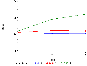
Just as in the case of proc glm it is often very useful to look at the graph of the means in order
to really understand the data. So, here is the code for creating the graphs in proc mixed that we were
able to obtain when using proc glm.
/* Proc Mixed does not have an out option in the lsmeans statement.  Instead we use
ODS to create the data set containing all the means. */
ods output LSMeans=means1;
proc mixed data=long;
  class exertype time;
  model pulse = exertype time exertype*time;
  repeated time / subject=id type=ar(1);
  lsmeans time*exertype;
run;

/* We print the dataset just to make sure that we have created the correct dataset. */
proc print data=means1;
run;

/* First we reset all the plot options to avoid any carry over from previous plotting procedures.  We use
a format statement in the proc gplot because the values for estimate have been assigned many decimal places that do not look
very nice when used as tick marks on the y-axis.  The format 8. means that we will allow there to be 8 digits for the
whole number and no decimal places.  This statement is included purely for cosmetic purposes and can easily be removed.
To understand all the plotting options used please refer to our webpage
on using proc gplot. */
goptions reset=all;
symbol1 c=blue v=star h=.8 i=j;
symbol2 c=red v=dot h=.8 i=j;
symbol3 c=green v=square h=.8 i=j;
axis1 order=(60 to 150 by 30) label=(a=90 'Means');
proc gplot data=means1;
  format estimate 8.;
  plot estimate*time=exertype / vaxis=axis1;
run;
quit;
Here is the graph.
Exercise example,
model 3 (time, diet and exertype)–Proc Glm
Looking at models including only diet or exertype separately does not answer all our questions.
We would also like to know if the
people on the low-fat diet who engage in running have lower pulse rates than the people participating
in the not low-fat diet who are not running. In order to address these types of questions we need to look at
a model that includes the interaction of diet and exertype. After all the analysis involving
the variance-covariance structures we will look at this model using both proc glm and proc mixed.
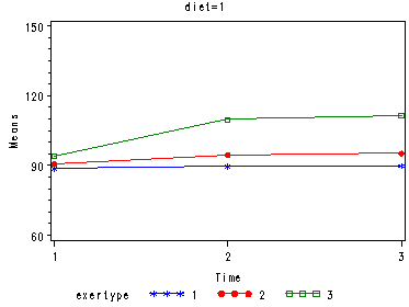
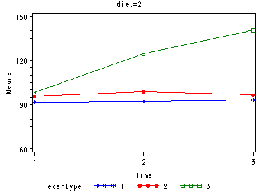
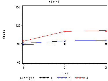
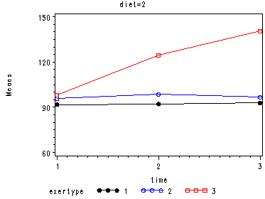
In the graph of exertype by diet we see that for the low-fat diet (diet=1) group the pulse
rate for the two exercise types: at rest and walking, are very close together, indeed they are
almost flat, whereas the running group has a higher pulse rate that increases over time. For the
not low-fat diet (diet=2) group the same two exercise types: at rest and walking, are also very close
together and almost flat. For this group, however, the pulse rate for the running group increases greatly
over time and the rate of increase is much steeper than the increase of the running group in the low-fat diet group.
The within subject tests indicate that there is a three-way interaction between diet, exertype and time. In other words, the pulse rate will depend on which diet you follow, the exercise type
you engage in and at what time during the exercise that you measure the pulse. The interactions of time and exertype and diet and exertype are also
significant as are the main effects of diet and exertype.
proc glm data=exercise;
 class diet exertype;
 model time1 time2 time3 = diet|exertype;
 repeated time 3 ;
run;
quit;
Looking at the graphs of exertype by diet.
Tests of Hypotheses for Between Subjects Effects

Source                     DF    Type III SS    Mean Square   F Value   Pr > F
DIET                        1    1261.877778    1261.877778     14.52   0.0008
EXERTYPE                    2    8326.066667    4163.033333     47.92   <.0001
DIET*EXERTYPE               2     815.755556     407.877778      4.69   0.0190
Error                      24    2085.200000      86.883333

Univariate Tests of Hypotheses for Within Subject Effects

Source                     DF    Type III SS    Mean Square   F Value   Pr > F
time                        2    2066.600000    1033.300000     31.72   <.0001
time*DIET                   2     192.822222      96.411111      2.96   0.0614
time*EXERTYPE               4    2723.333333     680.833333     20.90   <.0001
time*DIET*EXERTYPE          4     613.644444     153.411111      4.71   0.0028
Error(time)                48    1563.600000      32.575000
Creating Graphs for model 3 Using Proc Glm
proc glm data=exercise;
 class diet exertype;
 model time1 time2 time3 = diet|exertype;
 repeated time 3;
 lsmeans diet*exertype / out=means;
run;
quit;

proc print data=means;
run;

proc sort data=means out=sortdiet;
 by diet;
run;

goptions reset=all;
symbol1 c=blue v=star h=.8 i=j;
symbol2 c=red v=dot h=.8 i=j;
symbol3 c=green v=square h=.8 i=j;
axis1 order=(60 to 150 by 30) label=(a=90 'Means');
axis2 label=('Time') value=('1' '2' '3');
proc gplot data=sortdiet;
 by diet;
 plot lsmean*_name_ = exertype / vaxis=axis1 haxis=axis2;
run;
quit;
Exercise example,
model 3 (time, diet and exertype)–Proc Mixed
For the mixed model we will use the autoregressive heterogeneous variances variance-covariance structure
since we previously observed that this is the structure that appears to fit the data the best (see discussion
of variance-covariance structures). We do not expect to find a great change in which factors will be significant
but we do expect to have a model that has a better fit than the glm model.
The graphs are exactly the same as the glm model and we find that the same factors are significant. However, since
the model has a better fit we can be more confident in the estimate of the standard errors and therefore we can
be more confident in the tests and in the findings of significant factors. The model has a better fit than the
model only including exertype and time because both the -2Log Likelihood and the AIC has decrease dramatically.
The -2 Log Likelihood decreased from 579.8 for the model including only exertype and
time to 505.3
for the current model; the AIC decreased from 587.8 for the model including only exertype and time
to 513.3 for the current model.
The code for the mixed model

proc mixed data=long;
  class exertype diet time;
  model pulse = exertype|diet|time;
  repeated time / subject=id type=arh(1) ;
run;
Looking at the graphs of exertype by diet.
Covariance Parameter Estimates

Cov
Parm       Subject    Estimate
Var(1)     id          33.0864
Var(2)     id          73.5148
Var(3)     id          45.3847
ARH(1)     id           0.3610


           Fit Statistics
-2 Res Log Likelihood           505.3
AIC (smaller is better)         513.3
AICC (smaller is better)        513.9
BIC (smaller is better)         518.9


  Null Model Likelihood Ratio Test

    DF    Chi-Square      Pr > ChiSq
     3         10.65          0.0138


             Type 3 Tests of Fixed Effects

                       Num     Den
Effect                  DF      DF    F Value    Pr > F
exertype                 2      24      52.17    <.0001
diet                     1      24      15.81    0.0006
exertype*diet            2      24       5.11    0.0142
time                     2      48      30.82    <.0001
exertype*time            4      48      20.25    <.0001
diet*time                2      48       2.80    0.0709
exertype*diet*time       4      48       4.45    0.0039
Creating Graphs for model 3 Using Proc Mixed
/* Proc Mixed does not have an out option in the lsmeans statement.  Instead we use
ODS to create the data set containing all the means. */
ods output LSMeans = means;
proc mixed data=long;
  class exertype diet time;
  model pulse = exertype|diet|time;
  repeated time / subject=id type=arh(1) ;
  lsmeans time*diet*exertype;
run;
/* We print the dataset just to make sure that we have created the correct dataset. */
proc print data=means;
run;
proc sort data=means;
  by diet;
run;

/* First we reset all the plot options to avoid any carry over from previous plotting procedures.
We use a format statement in the proc gplot because the values for estimate have been assigned
many decimal places that do not look very nice when used as tick marks on the y-axis.  The format 8.
means that we will allow there to be 8 digits for the whole number and no decimal places.  This
statement is included purely for cosmetic purposes and can easily be removed.  To understand all
the plotting options used please refer to our webpage on using proc gplot. */

goptions reset=all;
symbol1 c=black v=dot i=j;
symbol2 c=blue v=circle i=j;
symbol3 c=red v=square i=j;
axis1 order=(60 to 150 by 30) label=(a=90 'Means');
proc gplot data=means;
  by diet;
  format estimate 8.;
  plot estimate*time=exertype / vaxis=axis1;
run;
quit;
Contrasts and interaction contrasts for model 3
From the graphs in the above analysis we see that the runners (exertype level 3) have a pulse rate that is
increases much quicker than the pulse rates of the two other groups. We would like to know if there is a
statistically significant difference between the changes over time in the pulse rate of the runners versus the
change over time in the pulse rate of the walkers and the “rest-ers” (the people at rest) across diet groups and
across time. Furthermore, we suspect
that there might be a difference in pulse rate over time and across exercise type between the two diet groups.
But to make matters even more
complicated we would like to test if the runners in the low fat diet group are statistically significantly different
from all the other groups (i.e. the runners in the non-low fat diet, the walkers and the
“rest-ers” in both diet groups).
Since we are being ambitious we also want to test if the runners in the low fat diet group (diet=1) are different from the runners
in the non-low fat diet group (diet=2). These contrasts are all
tested using the estimate statement in proc mixed.
If we would like to look at the differences among groups at each level of another variable we have to utilize
the lsmeans statement with the slice option. For example, we could test for differences among the
exertype groups at each level of diet across all levels of time; or we could test for differences in groups of
exertype for each time point across both levels of diet; we could also test for differences in groups of exertype
for each combination of time and diet levels.
proc mixed data=long;
  class diet exertype  time;
  model pulse = exertype|diet|time ;
  repeated time / subject=id type=arh(1) ;
  estimate 'exer 12 v 3' exertype  -.5 -.5 1; /* across time and across diet groups */
  estimate 'exer 1 v 2' exertype  -1 1 0; /* across time and across diet groups */
  estimate 'diet' diet  -1 1; /* across time and across exercise types */
  estimate 'diet 1v2 & exertype 12v3'
           diet*exertype -.5 -.5  1
                          .5  .5 -1;   /* across time only */
  estimate 'runners only, diet 1 v 2'  diet 1 -1
                            diet*exertype 0 0  1
			                  0 0 -1; /* across time only */
  lsmeans diet*exertype / slice=diet; /*testing for differences among exertype for each level of diet */
  lsmeans exertype*time / slice=time; /*differences in exertype for each time point*/
  lsmeans exertype*diet*time / slice=time*diet;
run;
quit;
             Type 3 Tests of Fixed Effects

                       Num     Den
Effect                  DF      DF    F Value    Pr > F

exertype                 2      24      52.17    <.0001
diet                     1      24      15.81    0.0006
diet*exertype            2      24       5.11    0.0142
time                     2      48      30.82    <.0001
exertype*time            4      48      20.25    <.0001
diet*time                2      48       2.80    0.0709
diet*exertype*time       4      48       4.45    0.0039


                                   Estimates

                                        Standard
Label                       Estimate       Error      DF    t Value    Pr > |t|

exer 12 v 3                  20.0500      1.9975      24      10.04      <.0001
exer 1 v 2                    4.3667      2.3066      24       1.89      0.0705
diet                          7.4889      1.8833      24       3.98      0.0006
diet 1v2 & exertype 12v3    -12.7667      3.9951      24      -3.20      0.0039
runners only, diet 1 v 2    -16.0000      3.2620      24      -4.91      <.0001


                            Least Squares Means

                                                    Standard
Effect              diet  exertype  time  Estimate     Error    DF  t Value

diet*exertype       1     1                89.3333    2.3066    24    38.73
diet*exertype       1     2                93.4667    2.3066    24    40.52
diet*exertype       1     3                 105.07    2.3066    24    45.55
diet*exertype       2     1                92.3333    2.3066    24    40.03
diet*exertype       2     2                96.9333    2.3066    24    42.03
diet*exertype       2     3                 121.07    2.3066    24    52.49
exertype*time             1         1      90.2000    1.8190    48    49.59
exertype*time             1         2      90.9000    2.7114    48    33.53
exertype*time             1         3      91.4000    2.1304    48    42.90
exertype*time             2         1      93.1000    1.8190    48    51.18
exertype*time             2         2      96.6000    2.7114    48    35.63
exertype*time             2         3      95.9000    2.1304    48    45.02
exertype*time             3         1      96.1000    1.8190    48    52.83
exertype*time             3         2       117.10    2.7114    48    43.19
exertype*time             3         3       126.00    2.1304    48    59.14
diet*exertype*time  1     1         1      88.6000    2.5724    48    34.44
diet*exertype*time  1     1         2      89.6000    3.8344    48    23.37
diet*exertype*time  1     1         3      89.8000    3.0128    48    29.81
diet*exertype*time  1     2         1      90.6000    2.5724    48    35.22
diet*exertype*time  1     2         2      94.6000    3.8344    48    24.67
diet*exertype*time  1     2         3      95.2000    3.0128    48    31.60
diet*exertype*time  1     3         1      94.0000    2.5724    48    36.54
diet*exertype*time  1     3         2       109.80    3.8344    48    28.64
diet*exertype*time  1     3         3       111.40    3.0128    48    36.98
diet*exertype*time  2     1         1      91.8000    2.5724    48    35.69
diet*exertype*time  2     1         2      92.2000    3.8344    48    24.05
diet*exertype*time  2     1         3      93.0000    3.0128    48    30.87
diet*exertype*time  2     2         1      95.6000    2.5724    48    37.16
diet*exertype*time  2     2         2      98.6000    3.8344    48    25.71
diet*exertype*time  2     2         3      96.6000    3.0128    48    32.06
diet*exertype*time  2     3         1      98.2000    2.5724    48    38.17
diet*exertype*time  2     3         2       124.40    3.8344    48    32.44
diet*exertype*time  2     3         3       140.60    3.0128    48    46.67

               Least Squares Means

Effect              diet  exertype  time  Pr > |t|

diet*exertype       1     1                 <.0001
diet*exertype       1     2                 <.0001
diet*exertype       1     3                 <.0001
diet*exertype       2     1                 <.0001
diet*exertype       2     2                 <.0001
diet*exertype       2     3                 <.0001
exertype*time             1         1       <.0001
exertype*time             1         2       <.0001
exertype*time             1         3       <.0001
exertype*time             2         1       <.0001
exertype*time             2         2       <.0001
exertype*time             2         3       <.0001
exertype*time             3         1       <.0001
exertype*time             3         2       <.0001
exertype*time             3         3       <.0001
diet*exertype*time  1     1         1       <.0001
diet*exertype*time  1     1         2       <.0001
diet*exertype*time  1     1         3       <.0001
diet*exertype*time  1     2         1       <.0001
diet*exertype*time  1     2         2       <.0001
diet*exertype*time  1     2         3       <.0001
diet*exertype*time  1     3         1       <.0001
diet*exertype*time  1     3         2       <.0001
diet*exertype*time  1     3         3       <.0001
diet*exertype*time  2     1         1       <.0001
diet*exertype*time  2     1         2       <.0001
diet*exertype*time  2     1         3       <.0001
diet*exertype*time  2     2         1       <.0001
diet*exertype*time  2     2         2       <.0001
diet*exertype*time  2     2         3       <.0001
diet*exertype*time  2     3         1       <.0001
diet*exertype*time  2     3         2       <.0001
diet*exertype*time  2     3         3       <.0001


                        Tests of Effect Slices

                                       Num     Den
Effect                diet    time      DF      DF    F Value    Pr > F

diet*exertype         1                  2      24      12.51    0.0002
diet*exertype         2                  2      24      44.77    <.0001
exertype*time                 1          2      48       2.63    0.0824
exertype*time                 2          2      48      25.83    <.0001
exertype*time                 3          2      48      77.98    <.0001
diet*exertype*time    1       1          2      48       1.13    0.3326
diet*exertype*time    1       2          2      48       7.53    0.0014
diet*exertype*time    1       3          2      48      13.92    <.0001
diet*exertype*time    2       1          2      48       1.57    0.2194
diet*exertype*time    2       2          2      48      19.76    <.0001
diet*exertype*time    2       3          2      48      77.39    <.0001
From the tests we see that there is a significant difference between the pulse rate over time of
the runners of the low fat diet and the runners of the non-low fat diet. The runners of the low
fat diet also have significantly different pulse rate from the pulse rate of all the other
groups (the runners of the non-low fat diet, the walkers and “rest-ers” of both diet groups).
The runners have a different pulse rate over time from the walkers and “rest-ers” combined.
The only time we do not have a significant results is when we look at the pulse rate of
the walkers and “rest-ers” over time. Here the test has a p-value of 0.0705 which exceeds
0.05 and thus it is not significant.
When looking at diet=1 and diet=2 separately across all time points we find that there is significant
differences in the exertype groups. At time=2 and time=3 there is also a significant difference between
exertype groups across both diets. There is not a significant differences between the exertype
groups when looking at time=1 and diet=1 nor is there
a significant differences among the groups when looking at time=1 and diet=2. For all other
combinations of diet and time levels there is a significant difference among the exertype groups.
It might be tempting to try and use the same type of estimate statements in proc glm in order to
perform similar types of contrasts. Unfortunately, the results of the estimate statement will be for
each of the dependent variable rather than across the repeated measure. Thus, it is not possible to test
any of the contrasts that we performed in proc mixed in the above analysis in proc glm using an
estimate statement since these contrasts are all done across time. In proc glm these
contrasts would be performed separately for each time point which is very different from the results
we obtained in proc mixed.
Unequally Spaced Time Points
Modeling Time as a Linear Predictor of Pulse
We have another study which is very similar to the one previously discussed except that
in this new study the pulse measurements were not taken at regular time points.
In this study a baseline pulse measurement was obtained at time = 0 for every individual
in the study. However, subsequent pulse measurements were taken at less
regular time intervals. The second pulse measurements were taken at approximately 2 minutes
(time = 120 seconds); the pulse measurement was obtained at approximately 5 minutes (time
= 300 seconds);
and the fourth and final pulse measurement was obtained at approximately 10 minutes (time
= 600
seconds). The data for this study is displayed below and it is available in the
study2 data file.
data study2;
  input id exertype diet pulse time;
cards;
1 1 1 90 0
1 1 1 92 228
1 1 1 93 296
1 1 1 93 639
2 1 1 90 0
2 1 1 92 56
2 1 1 93 434
2 1 1 93 538
3 1 1 97 0
3 1 1 97 150
3 1 1 94 295
3 1 1 94 541
4 1 1 80 0
4 1 1 82 121
4 1 1 83 256
4 1 1 83 575
5 1 1 91 0
5 1 1 92 161
5 1 1 91 252
5 1 1 91 526
6 1 2 83 0
6 1 2 83 73
6 1 2 84 320
6 1 2 84 570
7 1 2 87 0
7 1 2 88 40
7 1 2 90 325
7 1 2 90 730
8 1 2 92 0
8 1 2 94 205
8 1 2 95 276
8 1 2 95 761
9 1 2 97 0
9 1 2 99 57
9 1 2 96 244
9 1 2 96 695
10 1 2 100 0
10 1 2 97 143
10 1 2 100 296
10 1 2 100 722
11 2 1 86 0
11 2 1 86 83
11 2 1 84 262
11 2 1 84 566
12 2 1 93 0
12 2 1 103 116
12 2 1 104 357
12 2 1 104 479
13 2 1 90 0
13 2 1 92 191
13 2 1 93 280
13 2 1 93 709
14 2 1 95 0
14 2 1 96 112
14 2 1 100 219
14 2 1 100 367
15 2 1 89 0
15 2 1 96 96
15 2 1 95 339
15 2 1 95 639
16 2 2 84 0
16 2 2 86 92
16 2 2 89 351
16 2 2 89 508
17 2 2 103 0
17 2 2 109 196
17 2 2 114 213
17 2 2 120 634
18 2 2 92 0
18 2 2 96 117
18 2 2 101 227
18 2 2 101 614
19 2 2 97 0
19 2 2 98 70
19 2 2 100 295
19 2 2 100 515
20 2 2 102 0
20 2 2 104 165
20 2 2 103 302
20 2 2 103 792
21 3 1 93 0
21 3 1 98 100
21 3 1 110 396
21 3 1 115 498
22 3 1 98 0
22 3 1 104 104
22 3 1 112 310
22 3 1 117 518
23 3 1 98 0
23 3 1 105 148
23 3 1 118 208
23 3 1 121 677
24 3 1 87 0
24 3 1 122 171
24 3 1 127 320
24 3 1 133 633
25 3 1 94 0
25 3 1 110 57
25 3 1 116 268
25 3 1 119 657
26 3 2 95 0
26 3 2 126 163
26 3 2 143 382
26 3 2 147 501
27 3 2 100 0
27 3 2 126 70
27 3 2 140 347
27 3 2 148 737
28 3 2 103 0
28 3 2 124 61
28 3 2 140 263
28 3 2 143 588
29 3 2 94 0
29 3 2 135 164
29 3 2 130 353
29 3 2 137 560
30 3 2 99 0
30 3 2 111 114
30 3 2 140 362
30 3 2 148 501
;
run;
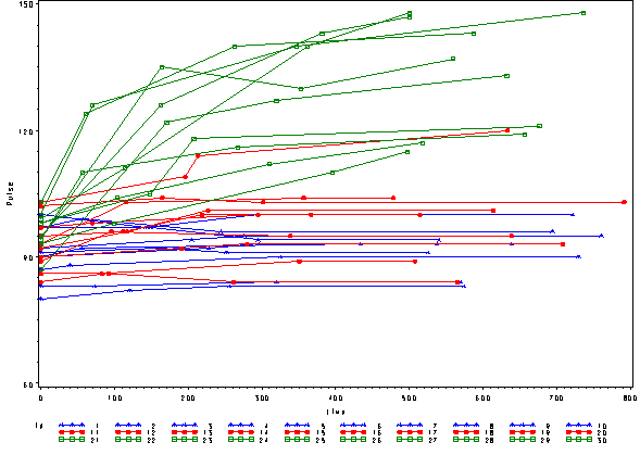
In order to get a better understanding of the data we will look at a scatter plot
of the data with lines connecting the points for each individual.
proc sort data=study2;
  by id time;
run;
goptions reset=all;
symbol1 c=blue v=star h=.8 i=j r=10;
symbol2 c=red v=dot h=.8 i=j r=10;
symbol3 c=green v=square h=.8 i=j r=10;
axis1 order=(60 to 150 by 30) label=(a=90 'Pulse');
proc gplot data=study2;
  plot pulse*time=id  / vaxis=axis1;
run;
This is a situation where multilevel modeling excels for the analysis of data
with irregularly spaced time points. The multilevel model with time
as a linear effect is illustrated in the following equations.
Level 1 (time): Pulse = β0j + β1j
(Time) + rij
Level 2 (person): β0j = γ00
+ γ01(Exertype) + u0j
Level 2 (person): β1j = γ10 + γ11(Exertype)
+ u1j
Substituting the level 2 model into the level 1 model we get the following single
equations. Note: The random components have been placed in square brackets.
Pulse = γ00 + γ01(Exertype)
+ γ10(Time) + γ11(Exertype*time) + [ u0j +
u1j(Time) + rij ]
Since this model contains both fixed and random components, it can be
analyzed in proc mixed as shown below.
*the linear model ;
proc mixed data=study2 covtest noclprint;
  class id exertype ;
  model pulse = time exertype time*exertype / solution outp=pred1r outpm = pred1f;
  random intercept time / subject = id;
run;
                  Covariance Parameter Estimates

                                     Standard         Z
Cov Parm      Subject    Estimate       Error     Value        Pr Z
Intercept     id          33.8894     13.3635      2.54      0.0056
time          id         0.000133    0.000080      1.66      0.0482
Residual                  32.4052      5.4327      5.96      <.0001

                           Solution for Fixed Effects

                                         Standard
Effect           exertype    Estimate       Error      DF    t Value    Pr > |t|
Intercept                      103.70      2.2884      27      45.31      <.0001
time                          0.05635    0.005405      27      10.43      <.0001
exertype         1           -12.6252      3.2262      60      -3.91      0.0002
exertype         2            -9.1144      3.2309      60      -2.82      0.0065
exertype         3                  0           .       .        .         .
time*exertype    1           -0.05477    0.007531      60      -7.27      <.0001
time*exertype    2           -0.04760    0.007711      60      -6.17      <.0001
time*exertype    3                  0           .       .        .         .

          Type 3 Tests of Fixed Effects

                  Num     Den
Effect             DF      DF    F Value    Pr > F
time                1      27      51.13    <.0001
exertype            2      60       8.15    0.0007
time*exertype       2      60      30.68    <.0001
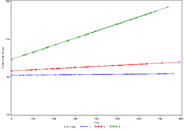
The output file pred1f contains the predicted values based on the
fixed part of the model. We can illustrate what the predicted values of
pulse look like using this model below.
goptions reset=all;
symbol1 c=blue v=star h=.8 i=j;
symbol2 c=red v=dot h=.8 i=j;
symbol3 c=green v=square h=.8 i=j;
axis1 order=(60 to 150 by 30) label=(a=90 'Predicted Pulse');
proc gplot data=pred1f;
  plot pred*time=exertype  /vaxis=axis1;
run;
quit;
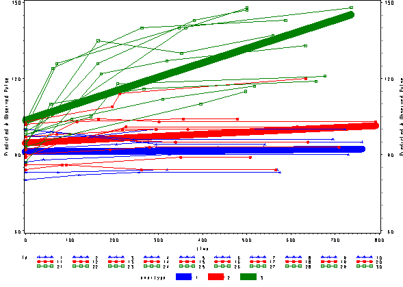
We can include the observed pulse as well and see that this model is not
fitting very well at all. The green line is fitting curved data with a
straight line.
proc sort data=pred1f;
  by time;
run;
goptions reset=all;
symbol1 c=blue  v=star   h=.8 i=j      w=10;
symbol2 c=red   v=dot    h=.8 i=j      w=10;
symbol3 c=green v=square h=.8 i=j      w=10;
symbol4 c=blue  v=star   h=.8 i=j      r=10;
symbol5 c=red   v=dot    h=.8 i=j      r=10;
symbol6 c=green v=square h=.8 i=j      r=10;
axis1 order=(60 to 150 by 30) label=(a=90 'Predicted and Observed Pulse');
proc gplot data=pred1f;
  plot pred*time=exertype / vaxis=axis1 ;
  plot2 pulse*time = id   / vaxis=axis1 ;;
run;
quit;
Modeling Time as a Quadratic Predictor of Pulse
To model the quadratic effect of time, we add time*time to
the model. We see that term is significant.
*the quadratic model ;
proc mixed data=study2 covtest noclprint;
  class id exertype;
  model pulse = time exertype time*exertype time*time / solution outp=pred2r outpm=pred2f ;
  random intercept time / subject = id;
run;

                Covariance Parameter Estimates

                                     Standard         Z
Cov Parm      Subject    Estimate       Error     Value        Pr Z
Intercept     id          33.2228     12.3961      2.68      0.0037
time          id         0.000151    0.000075      2.00      0.0226
Residual                  24.8148      4.2003      5.91      <.0001

                           Solution for Fixed Effects

                                         Standard
Effect           exertype    Estimate       Error      DF    t Value    Pr > |t|
Intercept                      101.68      2.2145      27      45.91      <.0001
time                          0.08777    0.008310      27      10.56      <.0001
exertype         1           -12.9233      3.0723      59      -4.21      <.0001
exertype         2            -9.3558      3.0757      59      -3.04      0.0035
exertype         3                  0           .       .        .         .
time*exertype    1           -0.05253    0.007332      59      -7.16      <.0001
time*exertype    2           -0.04690    0.007464      59      -6.28      <.0001
time*exertype    3                  0           .       .        .         .
time*time                    -0.00005    0.000011      27      -4.83      <.0001

          Type 3 Tests of Fixed Effects

                  Num     Den
Effect             DF      DF    F Value    Pr > F
time                1      27      55.38    <.0001
exertype            2      59       9.42    0.0003
time*exertype       2      59      30.48    <.0001
time*time           1      27      23.28    <.0001
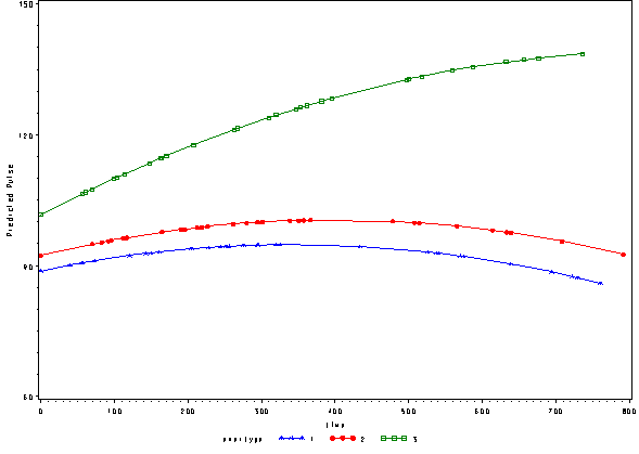
Below we see the predicted values from this model with the quadratic effect
of time.
* just predicted, fixed ;
proc sort data=pred2f;
  by time;
run;
goptions reset=all;
symbol1 c=blue v=star h=.8 i=j ;
symbol2 c=red v=dot h=.8 i=j ;
symbol3 c=green v=square h=.8 i=j ;
axis1 order=(60 to 150 by 30) label=(a=90 'Predicted Pulse');
proc gplot data=pred2f;
  plot pred*time=exertype      /vaxis=axis1 ;
run;
quit;
Again, we can plot the predicted values against the actual values of pulse.
We see that this model fits better, but it appears that the predicted values for
the green group have too little curvature and the red and blue group have too
much curvature.
* predicted vs. actual , fixed ;
proc sort data=pred2f;
  by time;
run;
goptions reset=all;
symbol1 c=blue  v=star   h=.8 i=j      w=10;
symbol2 c=red   v=dot    h=.8 i=j      w=10;
symbol3 c=green v=square h=.8 i=j      w=10;
symbol4 c=blue  v=star   h=.8 i=j      r=10;
symbol5 c=red   v=dot    h=.8 i=j      r=10;
symbol6 c=green v=square h=.8 i=j      r=10;
axis1 order=(60 to 150 by 30) label=(a=90 'Predicted and Observed Pulse');
proc gplot data=pred2f;
  plot pred*time=exertype / vaxis=axis1 ;
  plot2 pulse*time = id   / vaxis=axis1 ;;
run;
quit;
Modeling Time as a Quadratic Predictor of Pulse, Interacting by Exertype
We can include an interaction of time*time*exertype to indicate that the
different exercises not only show different linear trends over time, but that
they also show different quadratic trends over time, as shown below. The
time*time*exertype term is significant.
* quadratic model , model 3 ;
proc mixed data=study2 covtest noclprint;
  class id exertype;
  model pulse = time exertype time*exertype time*time time*time*exertype / solution outp=pred3r outpm=pred3f ;
  random intercept time / subject = id;
run;
                             Solution for Fixed Effects

                                              Standard
Effect                exertype    Estimate       Error      DF    t Value    Pr > |t|
Intercept                          98.0958      2.1923      27      44.75      <.0001
time                                0.1448     0.01065      27      13.60      <.0001
exertype              1            -7.2807      3.0989      57      -2.35      0.0223
exertype              2            -4.6201      3.1042      57      -1.49      0.1422
exertype              3                  0           .       .        .         .
time*exertype         1            -0.1393     0.01461      57      -9.53      <.0001
time*exertype         2            -0.1204     0.01472      57      -8.18      <.0001
time*exertype         3                  0           .       .        .         .
time*time                         -0.00014    0.000016      27      -9.17      <.0001
time*time*exertype    1           0.000139    0.000021      57       6.67      <.0001
time*time*exertype    2           0.000120    0.000021      57       5.60      <.0001
time*time*exertype    3                  0           .       .        .         .

             Type 3 Tests of Fixed Effects

                       Num     Den
Effect                  DF      DF    F Value    Pr > F
time                     1      27      96.49    <.0001
exertype                 2      57       2.83    0.0676
time*exertype            2      57      52.32    <.0001
time*time                1      27      84.11    <.0001
time*time*exertype       2      57      24.77    <.0001

* predicted vs. actual , fixed ;
proc sort data=pred3f;
  by time;
run;
goptions reset=all;
symbol1 c=blue  v=star   h=.8 i=j      w=10;
symbol2 c=red   v=dot    h=.8 i=j      w=10;
symbol3 c=green v=square h=.8 i=j      w=10;
symbol4 c=blue  v=star   h=.8 i=j      r=10;
symbol5 c=red   v=dot    h=.8 i=j      r=10;
symbol6 c=green v=square h=.8 i=j      r=10;
axis1 order=(60 to 150 by 30) label=(a=90 'Predicted and Observed Pulse');
proc gplot data=pred3f;
  plot pred*time=exertype / vaxis=axis1 ;
  plot2 pulse*time = id   / vaxis=axis1 ;;
run;
quit;
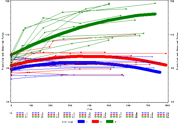
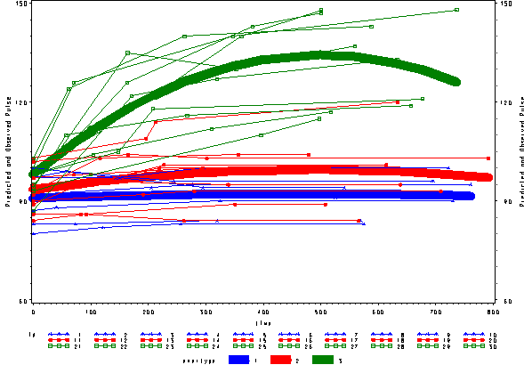
Below we see the predicted and actual values and see that this model fits
much better. The green curve hugs the data from the green group much
better and the blue and red groups are much flatter, fitting their data much
better as well.
For more information