
Mplus version 8 was used for these examples. All the files for this portion of this seminar can be downloaded here.
Confirmatory factor analysis (CFA) is a measurement model that estimates
continuous latent variables based on observed indicator variables (also called
manifest variables). The observed indicator variables may be either categorical
or continuous. One way to think about confirmatory factor analysis is that each
case has a “true score” on the (continuous) latent variable, and that each of
the observed values is a result of that “true score” plus measurement error. The
model attempts to estimate that “true score” based on the relationships among the observed values.
1.0 A measurement model for a single latent variable
The examples on this page use data on the attributes of a group of students
(see note at the bottom of the page for information on the source). The dataset (worland.dat)
contains 12 observed variables, which can be used to estimate four latent variables. The 12
observed variables have all been standardized to have a mean of zero and a
standard deviation of one. The four latent variables are students’
family “risk factors” (family), cognitive ability based on standardized tests (cognitive/cog),
achievement, that is, grades in school (achieve), and classroom adjustment based on ratings by
each student’s teacher (adjust). As a first step, we will estimate a model
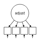
for a single latent variable. The diagram below shows the measurement
model for the adjustment latent variable (adjust). The observed
variables, represented as empty boxes are motivation (motiv),
extraversion (extra), harmony (harm) and stability (stabi).
The input file shown below estimates the model described above. In the model command block, the keyword by indicates that the
latent variable named before the by is measured by the manifest variables
listed after it. In order for a CFA model to be identified (i.e., the parameters will have a unique solution), one of two constraints must usually be imposed:
- one of the loadings is fixed to 1
- the latent factor variance is fixed to 1
The overall model fit will be the same whichever constraint is used. By default, Mplus will fix the loading of the first indicator listed after by in the model command block. We will see this in the output.
title: Measurement model for one latent variable
data:
file is worland.dat;

variable:
names are ppsych ses verbal vissp mem read arith spell motiv extra harm stabi;
usevariables are motiv extra harm stabi;

model:
adjust by motiv extra harm stabi;
The output based on this input file is shown below.
Measurement model for one latent variable

SUMMARY OF ANALYSIS

Number of groups                                                 1
Number of observations                                         500

Number of dependent variables                                    4
Number of independent variables                                  0
Number of continuous latent variables                            1

Observed dependent variables

  Continuous
   MOTIV       EXTRA       HARM        STABI

Continuous latent variables
   ADJUST

Estimator                                                       ML
Information matrix                                        OBSERVED
Maximum number of iterations                                  1000
Convergence criterion                                    0.500D-04
Maximum number of steepest descent iterations                   20

Input data file(s)
  worland.dat

Input data format  FREE

THE MODEL ESTIMATION TERMINATED NORMALLY

MODEL FIT INFORMATION

Number of Free Parameters                       12

Loglikelihood

          H0 Value                       -2481.245
          H1 Value                       -2371.942

Information Criteria

          Akaike (AIC)                    4986.489
          Bayesian (BIC)                  5037.065
          Sample-Size Adjusted BIC        4998.976
            (n* = (n + 2) / 24)

Chi-Square Test of Model Fit

          Value                            218.606
          Degrees of Freedom                     2
          P-Value                           0.0000

RMSEA (Root Mean Square Error Of Approximation)

          Estimate                           0.465
          90 Percent C.I.                    0.414  0.519
          Probability RMSEA <= .05           0.000

CFI/TLI

          CFI                                0.765
          TLI                                0.295

Chi-Square Test of Model Fit for the Baseline Model

          Value                            927.867
          Degrees of Freedom                     6
          P-Value                           0.0000

SRMR (Standardized Root Mean Square Residual)

          Value                              0.113

MODEL RESULTS

                                                    Two-Tailed
                    Estimate       S.E.  Est./S.E.    P-Value

 ADJUST   BY
    MOTIV              1.000      0.000    999.000    999.000
    EXTRA              0.211      0.053      4.002      0.000
    HARM               0.954      0.056     17.086      0.000
    STABI              0.722      0.050     14.582      0.000

 Intercepts
    MOTIV              0.000      0.045      0.000      1.000
    EXTRA              0.000      0.045      0.000      1.000
    HARM               0.000      0.045      0.000      1.000
    STABI              0.000      0.045      0.000      1.000

 Variances
    ADJUST             0.811      0.074     11.016      0.000

 Residual Variances
    MOTIV              0.187      0.041      4.505      0.000
    EXTRA              0.962      0.061     15.693      0.000
    HARM               0.259      0.040      6.499      0.000
    STABI              0.575      0.041     14.055      0.000

QUALITY OF NUMERICAL RESULTS

     Condition Number for the Information Matrix              0.385E-01
       (ratio of smallest to largest eigenvalue)

DIAGRAM INFORMATION

  Use View Diagram under the Diagram menu in the Mplus Editor to view the diagram.
  If running Mplus from the Mplus Diagrammer, the diagram opens automatically.

  Diagram output
    c:\temp\01-cfa.dgm
In the MODEL RESULTS section of the above output, the first block
of estimates labeled ADJUST BY contains the path coefficients (e.g. factor loadings) for the
relationship between the individual items and the latent variable. All of
the path coefficients (shown in the Estimates column) are positive,
indicating a positive relationship between the latent variable adjustment,
and our four observed measures of adjustment. In the far right column, we
can also see that each of the path coefficients is significantly different
from 0 (except for the first factor loading, which is fixed at 1). The subsequent blocks show the intercepts for the observed
variables (labeled Intercepts), the variance of the latent variable adjust (labeled
Variances), and the estimates of the error variance for each of the observed
variables (labeled Residual Variances). Note: all of the intercepts are estimated at zero because the indicator variables have all been standardized to have zero means. With unstandardized indicators, non-zero intercepts will typically be estimated.
2.0 A measurement model with multiple (correlated) latent variables
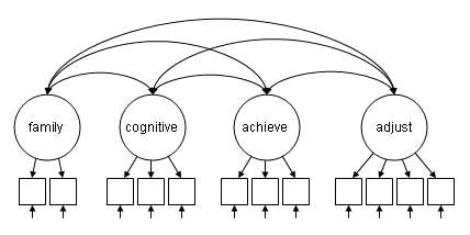
In this example, the model estimates all four latent variables at the
same time and allows the latent variables to covary without imposing additional
structure. A model with all of the latent variables allowed to covary is often run
as a precursor to a model with a more specific set of relationships among
the latent variables. The desired model is shown in the diagram
below. Note that the curved double-headed arrows denote covariances.
The input file for this model is similar to the last. This model contains
instructions for four latent variables, each measured by a series of observed
variables (e.g., family by ppsych ses;). By default, Mplus will estimate the covariances among all exogenous latent variables with each other, so we do not need to specify these covariances explicitly (e.g. family with cognitive achieve adjust).
title: Measurement model with correlations

data:
file is worland.dat;

variable:
names are ppsych ses verbal vissp mem read arith spell motiv extra harm stabi;

model:
adjust by motiv extra harm stabi;
family by ppsych ses;
cog by verbal vissp mem;
achieve by read arith spell;
The output based on this input file is shown below.
Measurement model with correlations

SUMMARY OF ANALYSIS

Number of groups                                                 1
Number of observations                                         500

Number of dependent variables                                   12
Number of independent variables                                  0
Number of continuous latent variables                            4

Observed dependent variables

  Continuous
   PPSYCH      SES         VERBAL      VISSP       MEM         READ
   ARITH       SPELL       MOTIV       EXTRA       HARM        STABI

Continuous latent variables
   ADJUST      FAMILY      COG         ACHIEVE


Estimator                                                       ML
Information matrix                                        OBSERVED
Maximum number of iterations                                  1000
Convergence criterion                                    0.500D-04
Maximum number of steepest descent iterations                   20

Input data file(s)
  worland.dat

Input data format  FREE

THE MODEL ESTIMATION TERMINATED NORMALLY

MODEL FIT INFORMATION

Number of Free Parameters                       42

Loglikelihood

          H0 Value                       -6745.325
          H1 Value                       -6445.272

Information Criteria

          Akaike (AIC)                   13574.649
          Bayesian (BIC)                 13751.663
          Sample-Size Adjusted BIC       13618.352
            (n* = (n + 2) / 24)

Chi-Square Test of Model Fit

          Value                            600.106
          Degrees of Freedom                    48
          P-Value                           0.0000

RMSEA (Root Mean Square Error Of Approximation)

          Estimate                           0.152
          90 Percent C.I.                    0.141  0.163
          Probability RMSEA <= .05           0.000

CFI/TLI

          CFI                                0.864
          TLI                                0.813

Chi-Square Test of Model Fit for the Baseline Model

          Value                           4124.707
          Degrees of Freedom                    66
          P-Value                           0.0000

SRMR (Standardized Root Mean Square Residual)

          Value                              0.063

MODEL RESULTS

                                                    Two-Tailed
                    Estimate       S.E.  Est./S.E.    P-Value

 ADJUST   BY
    MOTIV              1.000      0.000    999.000    999.000
    EXTRA              0.233      0.048      4.813      0.000
    HARM               0.857      0.042     20.295      0.000
    STABI              0.662      0.045     14.615      0.000

 FAMILY   BY
    PPSYCH             1.000      0.000    999.000    999.000
    SES               -1.107      0.115     -9.657      0.000

 COG      BY
    VERBAL             1.000      0.000    999.000    999.000
    VISSP              0.833      0.045     18.393      0.000
    MEM                0.972      0.044     22.326      0.000

 ACHIEVE  BY
    READ               1.000      0.000    999.000    999.000
    ARITH              0.842      0.034     24.840      0.000
    SPELL              0.954      0.027     35.622      0.000

 FAMILY   WITH
    ADJUST            -0.245      0.040     -6.099      0.000

 COG      WITH
    ADJUST             0.508      0.048     10.510      0.000
    FAMILY            -0.411      0.046     -8.852      0.000

 ACHIEVE  WITH
    ADJUST             0.567      0.051     11.102      0.000
    FAMILY            -0.363      0.044     -8.151      0.000
    COG                0.740      0.056     13.305      0.000

 Intercepts
    PPSYCH             0.000      0.045      0.000      1.000
    SES                0.000      0.045      0.000      1.000
    VERBAL             0.000      0.045      0.000      1.000
    VISSP              0.000      0.045      0.000      1.000
    MEM                0.000      0.045      0.000      1.000
    READ               0.000      0.045      0.000      1.000
    ARITH              0.000      0.045      0.000      1.000
    SPELL              0.000      0.045      0.000      1.000
    MOTIV              0.000      0.045      0.000      1.000
    EXTRA              0.000      0.045      0.000      1.000
    HARM               0.000      0.045      0.000      1.000
    STABI              0.000      0.045      0.000      1.000

 Variances
    ADJUST             0.901      0.070     12.842      0.000
    FAMILY             0.379      0.061      6.201      0.000
    COG                0.739      0.063     11.678      0.000
    ACHIEVE            0.897      0.064     14.002      0.000

 Residual Variances
    PPSYCH             0.619      0.053     11.681      0.000
    SES                0.534      0.055      9.652      0.000
    VERBAL             0.259      0.024     10.967      0.000
    VISSP              0.485      0.035     13.679      0.000
    MEM                0.300      0.026     11.643      0.000
    READ               0.101      0.014      7.142      0.000
    ARITH              0.362      0.027     13.612      0.000
    SPELL              0.181      0.016     11.387      0.000
    MOTIV              0.097      0.032      3.049      0.002
    EXTRA              0.949      0.060     15.702      0.000
    HARM               0.336      0.033     10.318      0.000
    STABI              0.604      0.042     14.269      0.000

QUALITY OF NUMERICAL RESULTS

     Condition Number for the Information Matrix              0.320E-02
       (ratio of smallest to largest eigenvalue)

DIAGRAM INFORMATION

  Use View Diagram under the Diagram menu in the Mplus Editor to view the diagram.
  If running Mplus from the Mplus Diagrammer, the diagram opens automatically.

  Diagram output
    c:\temp\02-cfa.dgm
Looking at the MODEL RESULTS section of the output, the first four blocks
of estimates give the path coefficients (e.g. factor loadings) for the relationship between the latent
variables and the observed variables (e.g., FAMILY BY). After the path coefficients for
the four latent variables, the covariances between the latent variables
(indicated using the keyword WITH) are shown. We see that the latent variable family (i.e.,
family risk factors) has a negative relationship with cog (cognitive
ability), achieve (academic achievement) and adjust (classroom
adjustment). Note that our input file does not explicitly include these
covariances; Mplus includes them by default.
3.0 Saving factor scores
In addition to the output file produced by Mplus, it is possible to save factor scores
for each case in a text file that can later be used by Mplus or read into
another statistical package. To do this the savedata command is added to the input file.
The file option gives the name of the file in which the factor scores
should be saved (i.e., scores.txt). Whenever the file option is used, all of the
variables used in the analysis are saved in an external file. The save = fscores;
option specifies that the factor scores should be saved in addition to the
variables used in estimation.
title: Saving factor scores

data:
file is worland.dat;

variable:
names are ppsych ses verbal vissp mem read arith spell motiv extra harm stabi;

model:
adjust by motiv extra harm stabi;
family by ppsych ses;
cog by verbal vissp mem;
achieve by read arith spell;

savedata:
file is scores.txt;
save = fscores;
The output file for this model contains all of the information contained in the output
for the previous model, plus additional output associated with the savedata command. This
additional output appears towards the end of the output file, and is shown below.
SAVEDATA INFORMATION

  Save file
    scores.txt

  Order and format of variables

    PPSYCH         F10.3
    SES            F10.3
    VERBAL         F10.3
    VISSP          F10.3
    MEM            F10.3
    READ           F10.3
    ARITH          F10.3
    SPELL          F10.3
    MOTIV          F10.3
    EXTRA          F10.3
    HARM           F10.3
    STABI          F10.3
    ADJUST         F10.3
    ADJUST_SE      F10.3
    FAMILY         F10.3
    FAMILY_SE      F10.3
    COG            F10.3
    COG_SE         F10.3
    ACHIEVE        F10.3
    ACHIEVE_SE     F10.3

  Save file format
    20F10.3

  Save file record length    10000
The additional output associated with the savedata
command block lists the variables in the order in which they appear in the saved
dataset. Note that the 12 observed variables used in estimation are listed
first. The next eight variables contain the factor scores associated
with each of the four latent variables, and the standard error of the factor scores.
Below the list of variables the name
of the file, and information on the format of the file are shown.
The file scores.txt is a text file that can be read by a large number of programs.
The first few lines of this file are shown below.
This file contains 20 variables, each in its own column. Based on the
information in the output file, we know that the first 12 columns contain
each student’s value on the 12 observed variables, and the final eight
columns are each student’s factor score for each of the four latent
variables and the standard error of the factor scores.
    -1.780     0.477    -0.790    -0.363     0.311    -0.349    -0.999    -0.657    -0.791    -0.496    -0.508    -0.314    -0.693     0.257    -0.318     0.326    -0.239     0.247    -0.509     0.217
     0.701    -0.605    -0.955    -0.769    -0.398    -0.452     0.820     0.878     0.175    -0.240    -0.416     0.352     0.055     0.257     0.452     0.326    -0.421     0.247    -0.013     0.217
     2.373    -1.697    -0.130    -0.391     0.146    -0.482     0.753    -0.569     1.447     0.293    -0.454     0.407     0.926     0.257     0.809     0.326    -0.333     0.247    -0.262     0.217
     0.149     0.140     1.752     2.141    -0.189    -0.314     0.573    -0.292    -0.117    -0.174    -0.567     0.260    -0.134     0.257    -0.315     0.326     0.536     0.247     0.011     0.217
    -0.599    -1.838     0.675    -0.144    -0.246    -0.201    -0.062    -0.102    -0.422     0.366    -1.007    -0.603    -0.498     0.257     0.253     0.326    -0.069     0.247    -0.123     0.217
Data source
The data for these examples is based on a correlation matrix published
in Worland et. al., 1984. Although the correlation matrix would have been
sufficient to specify these models, 500 cases were randomly drawn from the
distribution described by the published correlation matrix. The models above
do not necessarily match those specified in Worland et. al., 1984 they are
intended as examples only.
Worland, Julien, David G. Weeks, Cynthia L. Janes, and Strrock, Barbara D. (1984)
Intelligence, classroom behavior, and academic achievement in children at high
and low risk for psychopathology: A structural equation analysis. Journal of Abnormal Child Psychology
Vol. 12, No. 3, pp. 437-454.