
Mplus version 8 was used for these examples. All the files for this portion of this seminar can be downloaded here.
To illustrate longitudinal data analysis using Mplus we will use an example data set from Chapter 5 of Hox’s Multilevel Analysis: Techniques and Applications. The data set contains six GPAs for each subject measured at six time points, hence longitudinal. It has the hierarchical structure where measurements over the six time points are nested in students. Longitudinal modeling is a special case of multilevel modeling.
In Mplus a longitudinal model can be analyzed in one of the two ways: a univariate approach using the long format of the data (gpa_ch5_hox.dat) or a multivariate approach using the wide format (gpa_ch5_hox_wide.dat) of the same data. The approach using the long format is in the framework of multilevel modeling approach, while the approach using the wide format is in the framework of structural equation modeling (i.e., latent growth modeling). We will show both approaches in this section.
1.0 Longitudinal modeling in wide format, latent growth modeling
In order to perform a latent growth model, the data set will have to be restructured to
wide format:
student   gpa0   gpa1   gpa2   gpa3   gpa4   gpa5   job0   job1   job2   job3   job4   job5   highgpa   sex
   1      2.3    2.1      3      3      3    3.3      2      2      2      2      2      2      2.8      1
   2      2.2    2.5    2.6    2.6      3    2.8      2      3      2      2      2      2      2.5      0
   3      2.4    2.9      3    2.8    3.3    3.4      2      2      2      3      2      2      2.5      1
In the multivariate approach, we are more explicit about the latent variables
involved in the model. In this example, we have potentially two latent variables,
the random intercept and the random slope for time. We name them Intercept and Slope. We assume that the two latent
are normally distributed, and we are
interested in estimating the mean and variance of the two
variables. The model that we are going to run is the following:
$$
GPA_i = \Lambda \eta + \epsilon_i
$$
where \(\Lambda\) is a \(6 \times 2\) matrix of loadings for the intercept and slope, \(\eta\) is a \(2\times1\) vector of the latent intercept and slope with latent means \(\alpha_{intercept}\) and \(\alpha_{slope}\). The \(6 \times 1\) vector of residuals is defined by \(\epsilon\).
Here is a figure representing our latent growth model:
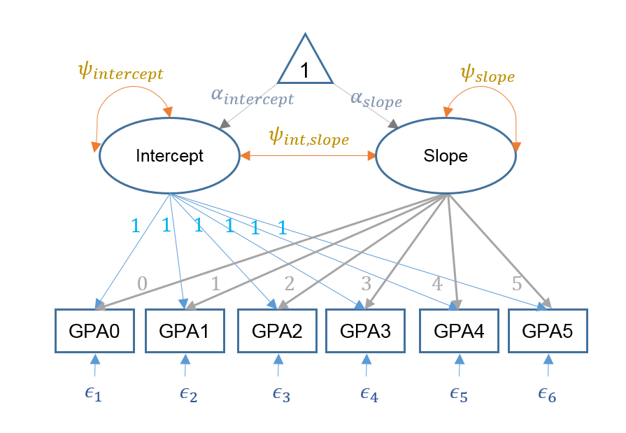
Multiplying out the equation above, the six equations for each time point defined for a person \(i\) and timepoint \(t\) is:
$$
GPA_{it} = Intercept_i + \lambda_t*Slope_i + e_{it}
$$
for \(t={0,1,2,3,4,5}\). Equivalently, the equation above can be spelled out with the corresponding six equations:
$$\begin{eqnarray}
GPA_{i0} & = & Intercept_{i} + 0*Slope_{i} + e_{i0} \\
GPA_{i1} & = & Intercept_{i} + 1*Slope_{i} + e_{i1} \\
GPA_{i2} & = & Intercept_{i} + 2*Slope_{i} + e_{i2} \\
GPA_{i3} & = & Intercept_{i} + 3*Slope_{i} + e_{i3} \\
GPA_{i4} & = & Intercept_{i} + 4*Slope_{i} + e_{i4} \\
GPA_{i5} & = & Intercept_{i} + 5*Slope_{i} + e_{i5}
\end{eqnarray}
$$
where the (symmetric) variance covariance matrix of the intercept and slope is defined as:
$$
\mathbf{\Psi} =
\begin{bmatrix}
\psi_{intercept} & \\
\psi_{int,slope} & \psi_{slope}
\end{bmatrix}
$$
A technical point is that in the multilevel approach, the
residual variance is homogeneous across all the time points. In order to match results to the multilevel model, we will also fix the residual variance to be the same across all the six time points.
title: Wide data format with random intercept

data:
    file is gpa_ch5_hox_wide.dat;

variable:
    names are student admitted gpa0 gpa1 gpa2 gpa3 gpa4 gpa5
    highgpa job0 job1 job2 job3 job4 job5 sex;
    missing are all (-9999);
    usevariables are  gpa0 gpa1 gpa2 gpa3 gpa4 gpa5;

analysis: estimator = ml;

model:
    i s | gpa0@0 gpa1@1 gpa2@2 gpa3@3 gpa4@4 gpa5@5;
    gpa0 - gpa5 (1); !fix the residual variance to be same across time points
MODEL RESULTS Two-Tailed Estimate S.E. Est./S.E. P-Value I | GPA0 1.000 0.000 999.000 999.000 GPA1 1.000 0.000 999.000 999.000 GPA2 1.000 0.000 999.000 999.000 GPA3 1.000 0.000 999.000 999.000 GPA4 1.000 0.000 999.000 999.000 GPA5 1.000 0.000 999.000 999.000 S | GPA0 0.000 0.000 999.000 999.000 GPA1 1.000 0.000 999.000 999.000 GPA2 2.000 0.000 999.000 999.000 GPA3 3.000 0.000 999.000 999.000 GPA4 4.000 0.000 999.000 999.000 GPA5 5.000 0.000 999.000 999.000 S WITH I -0.001 0.002 -0.834 0.404 Means I 2.599 0.018 141.947 0.000 S 0.106 0.006 18.111 0.000 Intercepts GPA0 0.000 0.000 999.000 999.000 GPA1 0.000 0.000 999.000 999.000 GPA2 0.000 0.000 999.000 999.000 GPA3 0.000 0.000 999.000 999.000 GPA4 0.000 0.000 999.000 999.000 GPA5 0.000 0.000 999.000 999.000 Variances I 0.045 0.007 6.599 0.000 S 0.004 0.001 6.387 0.000 Residual Variances GPA0 0.042 0.002 20.000 0.000 GPA1 0.042 0.002 20.000 0.000 GPA2 0.042 0.002 20.000 0.000 GPA3 0.042 0.002 20.000 0.000 GPA4 0.042 0.002 20.000 0.000 GPA5 0.042 0.002 20.000 0.000
2.0 Longitudinal modeling in wide format, without constraining the error variances
Now let’s rerun our previous example, but relax our assumption
on residual variance. In this example, we allow the residual variance across the
six time points to be different from each other. To this end, we just simply
comment out last line of the code in which we constrain the residual variance to
be the same. The point is that this approach in wide format gives us more
flexibility in modeling besides a different angle to look at the same model.
title: Wide data format without constraining the error variances

data:
    file is gpa_ch5_hox_wide.dat;

variable:
    names are student admitted gpa0 gpa1 gpa2 gpa3 gpa4 gpa5
    highgpa job0 job1 job2 job3 job4 job5 sex;
    missing are all (-9999);
    usevariables are  gpa0 gpa1 gpa2 gpa3 gpa4 gpa5;

analysis:
    estimator = ml;

model:
    i s | gpa0@0 gpa1@1 gpa2@2 gpa3@3 gpa4@4 gpa5@5;
    s@0;
   !gpa0 - gpa5 (1);

MODEL RESULTS

                                                    Two-Tailed
                    Estimate       S.E.  Est./S.E.    P-Value

 I        |
    GPA0               1.000      0.000    999.000    999.000
    GPA1               1.000      0.000    999.000    999.000
    GPA2               1.000      0.000    999.000    999.000
    GPA3               1.000      0.000    999.000    999.000
    GPA4               1.000      0.000    999.000    999.000
    GPA5               1.000      0.000    999.000    999.000

 S        |
    GPA0               0.000      0.000    999.000    999.000
    GPA1               1.000      0.000    999.000    999.000
    GPA2               2.000      0.000    999.000    999.000
    GPA3               3.000      0.000    999.000    999.000
    GPA4               4.000      0.000    999.000    999.000
    GPA5               5.000      0.000    999.000    999.000

 S        WITH
    I                  0.002      0.002      1.565      0.118

 Means
    I                  2.598      0.018    141.886      0.000
    S                  0.106      0.005     20.317      0.000

 Intercepts
    GPA0               0.000      0.000    999.000    999.000
    GPA1               0.000      0.000    999.000    999.000
    GPA2               0.000      0.000    999.000    999.000
    GPA3               0.000      0.000    999.000    999.000
    GPA4               0.000      0.000    999.000    999.000
    GPA5               0.000      0.000    999.000    999.000

 Variances
    I                  0.035      0.007      4.937      0.000
    S                  0.003      0.001      5.593      0.000

 Residual Variances
    GPA0               0.080      0.010      8.049      0.000
    GPA1               0.071      0.008      8.518      0.000
    GPA2               0.054      0.006      9.020      0.000
    GPA3               0.029      0.003      8.486      0.000
    GPA4               0.015      0.003      5.589      0.000
    GPA5               0.016      0.004      4.336      0.000
3.0 Longitudinal modeling in long format – random intercept model
When the data set is in long format, it contains multiple rows per subject. In this example, each student has at most six rows of data coming
from the measurements over the six time points. Here are observations of some of the variables for the first three subjects from the data set.
    student   time   gpa   job   sex
          1      0   2.3     2     1
          1      1   2.1     2     1
          1      2     3     2     1
          1      3     3     2     1
          1      4     3     2     1
          1      5   3.3     2     1
          2      0   2.2     2     0
          2      1   2.5     3     0
          2      2   2.6     2     0
          2      3   2.6     2     0
          2      4     3     2     0
          2      5   2.8     2     0
          3      0   2.4     2     1
          3      1   2.9     2     1
          3      2     3     2     1
          3      3   2.8     3     1
          3      4   3.3     2     1
          3      5   3.4     2     1
Our first multilevel model will be that GPA is a linearly related to time. The intercept is random, meaning it could change across subjects, but the slope of time is fixed, meaning the effect of time is the same across all the subjects. Mathematically, here is our first model:
$$\begin{eqnarray}
L1&: & GPA_{it} & = & \beta_{0i} + \beta_{1i}*TIME_{it} + e_{it} \\
L2&: & \beta_{0i} & = & \gamma_{00} + u_{0i} \\
&& \beta_{1i} & = & \gamma_{10}
\end{eqnarray}$$
where \(i\) stands for individual and \(t\) stands for time.
We also need to specify the nesting structure. The key words here for
describing the nesting structures are cluster, within and
between. A variable is a within variable if it is time-varying, such as the
job status. A variable is a between variable if it is not time-vary, such as
student’s gender. We specify the type of analysis to be twolevel and
random for running a longitudinal model. The model statement is very minimal
since the default model is a random intercept model.
title:  Long data format with random intercept

data:
    file is gpa_ch5_hox.dat;

variable:
    names are student highgpa gpa job admitted occas time sex;
    missing are all (-9999);
    usevariables are gpa time;
    cluster = student;
    within = time;

analysis:
    type = twolevel random;
    estimator = ml; !default is mlr

model:
    %within%
    gpa on time;
    %between%
    gpa;


SUMMARY OF ANALYSIS

Number of groups                                                 1
Number of observations                                        1200

Number of dependent variables                                    1
Number of independent variables                                  1
Number of continuous latent variables                            0

Observed dependent variables

  Continuous
   GPA

Observed independent variables
   TIME

Variables with special functions

  Cluster variable      STUDENT

  Within variables
   TIME

Estimator                                                       ML
Information matrix                                        OBSERVED
Maximum number of iterations                                   100
Convergence criterion                                    0.100D-05
Maximum number of EM iterations                                500
Convergence criteria for the EM algorithm
  Loglikelihood change                                   0.100D-02
  Relative loglikelihood change                          0.100D-05
  Derivative                                             0.100D-03
Minimum variance                                         0.100D-03
Maximum number of steepest descent iterations                   20
Maximum number of iterations for H1                           2000
Convergence criterion for H1                             0.100D-03
Optimization algorithm                                         EMA

Input data file(s)
  gpa_ch5_hox.dat
Input data format  FREE


SUMMARY OF DATA

     Number of missing data patterns             1
     Number of clusters                        200

     Average cluster size        6.000

     Estimated Intraclass Correlations for the Y Variables

                Intraclass
     Variable  Correlation

     GPA          0.411

COVARIANCE COVERAGE OF DATA

Minimum covariance coverage value   0.100

     PROPORTION OF DATA PRESENT


           Covariance Coverage
              GPA           TIME
              ________      ________
 GPA            1.000
 TIME           1.000         1.000

THE MODEL ESTIMATION TERMINATED NORMALLY

MODEL FIT INFORMATION

Number of Free Parameters                        4

Loglikelihood

          H0 Value                        -196.825
          H1 Value                        -196.825

Information Criteria

          Akaike (AIC)                     401.649
          Bayesian (BIC)                   422.009
          Sample-Size Adjusted BIC         409.304
            (n* = (n + 2) / 24)

Chi-Square Test of Model Fit

          Value                              0.000
          Degrees of Freedom                     0
          P-Value                           1.0000

RMSEA (Root Mean Square Error Of Approximation)

          Estimate                           0.000

CFI/TLI

          CFI                                1.000
          TLI                                1.000

Chi-Square Test of Model Fit for the Baseline Model

          Value                            519.807
          Degrees of Freedom                     1
          P-Value                           0.0000

SRMR (Standardized Root Mean Square Residual)

          Value for Within                   0.000
          Value for Between                  0.000

MODEL RESULTS

                                                    Two-Tailed
                    Estimate       S.E.  Est./S.E.    P-Value

Within Level

 GPA        ON
    TIME               0.106      0.004     26.109      0.000

 Residual Variances
    GPA                0.058      0.003     22.361      0.000

Between Level

 Means
    GPA                2.599      0.022    120.047      0.000

 Variances
    GPA                0.063      0.007      8.661      0.000

QUALITY OF NUMERICAL RESULTS

     Condition Number for the Information Matrix              0.126E-01
       (ratio of smallest to largest eigenvalue)

DIAGRAM INFORMATION

  Mplus diagrams are currently not available for multilevel analysis.
  No diagram output was produced.
4.0 Longitudinal modeling in long format – random intercept and random slope model
Our second multilevel model is a much more complicated model in which
we allow both a random intercept and random slope of time on top of a more involved
level-1 model where we add a new level-1 predictor variable, job. The
random intercept is in turn of linear function of between variable, sex
and highgpa. Mathematically, here is our second model:
$$\begin{eqnarray}
L1&: & GPA_{it} & = & \beta_{0i} + \beta_{1i}*TIME + \beta_{2t}*JOB + e_{it} \\
L2&: & \beta_{0i} & = & \gamma_{00} + \gamma_{01}*HIGHGPA + \gamma_{02}*SEX + u_{0i} \\
&& \beta_{1i} & = & \gamma_{10} + u_{1i}
\end{eqnarray}$$
Let’s look at the model statement to see what has been added. There are two lines
on the within statement. The first, gpa on job, indicates that we want a random
intercept and a fixed effect for job. On the next line, we request a random slope
that will be predicted by time. For the between part of the model, we will use
highgpa and sex as predictors. Because we have different predictor variables for
the intercept and slope, we will not have any cross-level interactions. On the
last line, we allow the intercept to be correlated with the slope.
title: Long data format with random intercept and random slope

data:
    file is gpa_ch5_hox.dat;

variable:
    names are student highgpa gpa job admitted occas time sex;
    missing are all (-9999);
    usevariables are gpa time job student highgpa  sex;
    cluster = student;
    within = time job;
    between = highgpa  sex;

analysis:
    type = twolevel random;
    estimator=ml; !default is mlr

model:
  %within%
    gpa on job;
    s | gpa on time;
  %between%
    gpa on highgpa sex;
    gpa with s;

SUMMARY OF ANALYSIS

Number of groups                                                 1
Number of observations                                        1200

Number of dependent variables                                    1
Number of independent variables                                  4
Number of continuous latent variables                            1

Observed dependent variables

  Continuous
   GPA

Observed independent variables
   TIME        JOB         HIGHGPA     SEX

Continuous latent variables
   S

Variables with special functions

  Cluster variable      STUDENT

  Within variables
   TIME        JOB

  Between variables
   HIGHGPA     SEX

Estimator                                                       ML
Information matrix                                        OBSERVED
Maximum number of iterations                                   100
Convergence criterion                                    0.100D-05
Maximum number of EM iterations                                500
Convergence criteria for the EM algorithm
  Loglikelihood change                                   0.100D-02
  Relative loglikelihood change                          0.100D-05
  Derivative                                             0.100D-03
Minimum variance                                         0.100D-03
Maximum number of steepest descent iterations                   20
Maximum number of iterations for H1                           2000
Convergence criterion for H1                             0.100D-03
Optimization algorithm                                         EMA

Input data file(s)
  gpa_ch5_hox.dat
Input data format  FREE

SUMMARY OF DATA

     Number of missing data patterns             1
     Number of clusters                        200

COVARIANCE COVERAGE OF DATA

Minimum covariance coverage value   0.100

     PROPORTION OF DATA PRESENT

           Covariance Coverage
              GPA           TIME          JOB           HIGHGPA       SEX
              ________      ________      ________      ________      ________
 GPA            1.000
 TIME           1.000         1.000
 JOB            1.000         1.000         1.000
 HIGHGPA        1.000         1.000         1.000         1.000
 SEX            1.000         1.000         1.000         1.000         1.000

THE MODEL ESTIMATION TERMINATED NORMALLY

MODEL FIT INFORMATION

Number of Free Parameters                        9

Loglikelihood

          H0 Value                         -90.102

Information Criteria

          Akaike (AIC)                     198.205
          Bayesian (BIC)                   244.016
          Sample-Size Adjusted BIC         215.428
            (n* = (n + 2) / 24)

MODEL RESULTS

                                                    Two-Tailed
                    Estimate       S.E.  Est./S.E.    P-Value

Within Level

 GPA        ON
    JOB               -0.120      0.018     -6.684      0.000

 Residual Variances
    GPA                0.042      0.002     19.894      0.000

Between Level

 GPA        ON
    HIGHGPA            0.090      0.026      3.393      0.001
    SEX                0.117      0.032      3.641      0.000

 GPA      WITH
    S                 -0.003      0.002     -1.645      0.100

 Means
    S                  0.104      0.006     18.491      0.000

 Intercepts
    GPA                2.527      0.093     27.195      0.000

 Variances
    S                  0.004      0.001      6.060      0.000

 Residual Variances
    GPA                0.039      0.006      6.264      0.000

QUALITY OF NUMERICAL RESULTS

     Condition Number for the Information Matrix              0.523E-03
       (ratio of smallest to largest eigenvalue)

DIAGRAM INFORMATION

  Mplus diagrams are currently not available for multilevel analysis.
  No diagram output was produced.