
Negative binomial regression is for modeling count variables, usually for
over-dispersed count outcome variables.
Please note: The purpose of this
page is to show how to use various data analysis commands. It does not cover
all aspects of the research process which researchers are expected to do. In
particular, it does not cover data cleaning and checking, verification of
assumptions, model diagnostics or potential follow-up analyses.
This page was updated using SPSS 19.
Examples of negative binomial regression
Example 1. School administrators study the attendance behavior of high
school juniors at two schools. Predictors of the number of days of absence
include the type of program in which the student is enrolled and a standardized
test in math.
Example 2. A health-related researcher is studying the number of hospital
visits in past 12 months by senior citizens in a community based on the
characteristics of the individuals and the types of health plans under which
each one is covered.
Description of the data
Let’s pursue Example 1 from above.
We have attendance data on 314 high school juniors from two urban high
schools in the file https://stats.idre.ucla.edu/wp-content/uploads/2016/02/nb_data.sav. The response
variable of interest is days absent, daysabs. The variable math
is the standardized math score for each student. The variable prog is a
three-level nominal variable indicating the type of instructional program in
which the student is enrolled.
Let’s look at the data. It is always a good idea to start with descriptive
statistics and plots.
get file "D:\data\nb_data.sav".

descriptives variables = daysabs math.
graph /histogram daysabs.
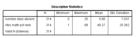
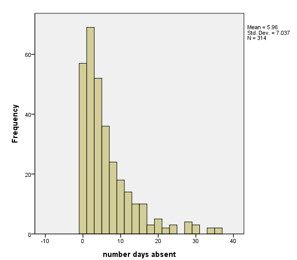
Each variable has 314 valid observations and their distributions seem quite reasonable. The unconditional mean of our outcome variable is much lower than its variance.
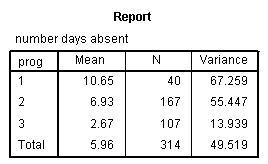
Let’s continue with our description of the variables in this dataset. The table below shows the average numbers of days absent by program type and seems to suggest that program type is a good candidate for predicting the number of days absent, our outcome variable, because the mean value of the outcome appears to vary by
prog. The variances within each level of prog are higher than the
means within each level. These are the conditional means and variances. These
differences suggest that over-dispersion is present and that a Negative Binomial
model would be appropriate.
means tables=daysabs by prog
  /cells mean count var.
Analysis methods you might consider
Below is a list of some analysis methods you may have
encountered. Some of the methods listed are quite reasonable, while others have
either fallen out of favor or have limitations.
- Negative binomial regression – Negative binomial regression can be used
for over-dispersed count data, that is when the conditional variance exceeds
the conditional mean. It can be considered as a generalization of Poisson
regression since it has the same mean structure as Poisson regression and it
has an extra parameter to model the over-dispersion. If the conditional
distribution of the outcome variable is over-dispersed, the confidence
intervals for the Negative binomial regression are likely to be narrower as
compared to those from a Poisson regression model. - Poisson regression – Poisson regression is often used for modeling count
data. Poisson regression has a number of extensions useful for count models. - Zero-inflated regression model – Zero-inflated models attempt to account
for excess zeros. In other words, two kinds of zeros are thought to exist
in the data, “true zeros” and “excess zeros”. Zero-inflated models estimate
two equations simultaneously, one for the count model and one for the excess
zeros. - OLS regression – Count outcome variables are sometimes log-transformed
and analyzed using OLS regression. Many issues arise with this approach,
including loss of data due to undefined values generated by taking the log
of zero (which is undefined), as well as the lack of capacity to model the
dispersion.
Negative binomial regression analysis
Below we use the genlin command to estimate a negative binomial regression
model. We use the SPSS keyword by to indicate that the variable
that follows is a categorical predictor, and we use the SPSS keyword with
to indicate that the variable that follow is a continuous predictor. We
use the (order = descending) option to use the first level of the
variable prog as the reference group. On the model
subcommand, we again list the predictor variables. We also indicate that
the distribution to be used is negbin (negative binomial) and the link is
a log link. By default, SPSS will not estimate the dispersion parameter.
Because we wish for this to be estimated, we specified (MLE) after our
distribution.
SPSS provides many output tables, so we will interrupt the output to
explain a few tables at a time.
genlin daysabs by prog (order = descending) with math
/model prog math distribution = negbin(MLE) link=log.
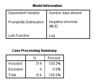
In the first two tables above, we see that the probability
distribution used was negative binomial, the link function was log, and
that all 314 cases were used in the analysis. We then see information on the distribution of the categorical
predictor variable, as well as information on the distribution of the
dependent variable and the continuous predictor variable.
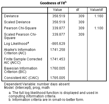
The table above provides several indices of the goodness of fit of the
model. These measures can be used to compare models.
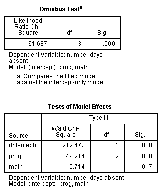
The tables above provide tests of the model as a whole (Omnibus Test). The
likelihood ratio chi-square provides a test of the overall model comparing this
model to a model without any predictors (a “null” model). We can see that our
model is a significant improvement over such a model by looking at the p-value
of this test.
In the Tests of Model Effects table, we see that each of the predictors
is statistically significant. The table includes the two degree of
freedom test of prog, which indicates that as a whole, the variable
prog is a significant predictor of dayabs.
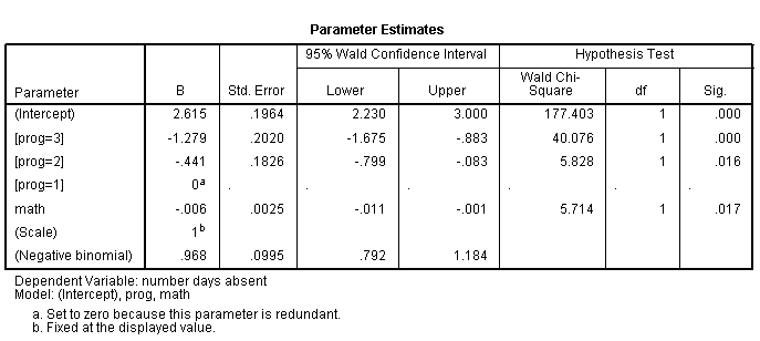
The table Parameter Estimates contains the negative binomial
regression coefficients for each of the predictor variables along with their standard errors,
Wald chi-square values, p-values and 95% confidence intervals for the coefficients.
Both of the dummy variables for the variable
prog are statistically significant. Compared to level 1 of
prog, the expected log count for level 2 decreases by 0.44.
Compared to level 1 of prog, the expected log count of 3.prog
decreases by 1.28. The variable math has a coefficient of -0.006, which
is statistically significant. This means that for each one-unit
increase on math, the expected log count of the number of days absent
decreases by 0.006 day.
Additionally, there is an estimate of the dispersion coefficient, (Negative
binomial). A Poisson model is one in which this value is constrained to
zero. In this example, the parameter’s 95% confidence interval does not include
zero, suggesting that the negative binomial model form is more appropriate than
the Poisson. An estimate greater than zero suggests over-dispersion (variance
greater than mean). An estimate less than zero suggests under-dispersion, which
is very rare.
If you would like the results displayed as incident rate ratios, you can use the
(exponentiated) option on the print subcommand after solution.
genlin daysabs by prog (order = descending) with math
/model prog math distribution = negbin(MLE) link=log
/print solution (exponentiated).
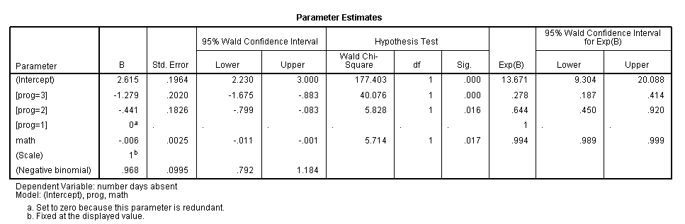
Looking at the Exp(B) column in the table above indicates that the
incident rate for prog=2 is 0.64 times the incident rate for the
reference group (prog=1). Likewise, the incident rate for prog=3
is 0.28 times the incident rate for the reference group holding the other
variables constant. The percent change in the incident rate of daysabs is
a 1% decrease for every unit increase in math.
The form of the model equation for negative binomial regression is the same
as that for Poisson regression. The log of the outcome is predicted with a
linear combination of the predictors:
log(daysabs) = Intercept + b1(prog=2) + b2(prog=3)
+ b3math.
This implies:
daysabs = exp(Intercept + b1(prog=2) + b2(prog=3)+
b3math) = exp(Intercept) * exp(b1(prog=2)) * exp(b2(prog=3))
* exp(b3math)
The coefficients have an additive effect in the log(y) scale and the
IRR have a multiplicative effect in the y scale. The overdispersion
parameter alpha in negative binomial regression does not effect the
expected counts, but it does effect the estimated variance of the expected
counts.
For additional information on the various metrics in which the results can be
presented, and the interpretation of such, please see Regression Models for
Categorical Dependent Variables Using Stata, Second Edition by J. Scott Long
and Jeremy Freese (2006).
For assistance in further understanding the model, we can use the emmeans
subcommand. Below we use the emmeans subcommand to calculate the predicted number of events at each level of
prog, holding all other variables (in this example, math) in the
model at their means.
genlin daysabs by prog (order = descending) with math
/model prog math distribution = negbin(MLE) link=log
/emmeans tables = prog scale = original.
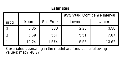
In the output above, we see that the predicted number of events (e.g., days
absent) for level 1
of prog is about 10.24, holding math at its mean. The predicted
number of events for level 2 of prog is lower at 6.59, and the
predicted number of events for level 3 of prog is about 2.85.
Below we will obtain the predicted number of events while holding math
at 20, then 40.
genlin daysabs by prog (order = descending) with math
/model prog math distribution = negbin(MLE) link=log
/emmeans control = math (20)
/emmeans control = math (40).
< some output omitted >
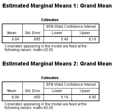
The tables above show that with prog at its observed values and math
held at 20 for all observations, the average predicted count (or average number of
days absent) is about 6.84; when math = 40, the average predicted count is about
6.06. If we compare the predicted counts at any two levels of math, like math =
20 and math = 40, we can see that the ratio is (6.06/6.84) = 0.89. This matches
the IRR of 0.994 for a 20 unit change: 0.994^20 = 0.89.
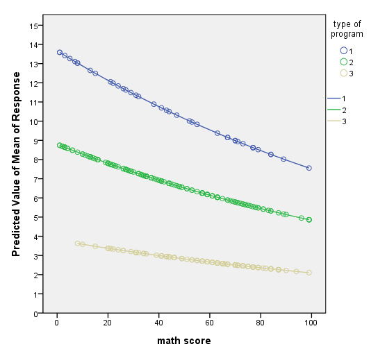
You can graph the predicted number of events with the commands below.
The graph indicates that the most awards are predicted for those in program
type 1, especially if the student has a high math score. The lowest number
of predicted awards is for those students in program type 3.
genlin daysabs by prog (order = descending) with math
/model prog math distribution = negbin(MLE) link=log
/save meanpred (mean_values).

GGRAPH
  /GRAPHDATASET NAME="graphdataset" VARIABLES=math mean_values prog
  /GRAPHSPEC SOURCE=INLINE.
BEGIN GPL
SOURCE: s=userSource(id("graphdataset"))
DATA: math=col(source(s), name("math"))
DATA: mean_values=col(source(s), name("mean_values"))
DATA: prog=col(source(s), name("prog"), unit.category())
GUIDE: axis(dim(1), label("math score"))
GUIDE: axis(dim(2), label("Predicted Value of Mean of Response"), delta(1))
GUIDE: legend(aesthetic(aesthetic.color.exterior), label("type of program"))
SCALE:  linear(dim(1), min(0), max(100))
SCALE:  linear(dim(2), min(0), max(14))
SCALE: cat(aesthetic(aesthetic.color.exterior), include("1.00", "2.00", "3.00"))
ELEMENT: point(position(math*mean_values), color.exterior(prog))
ELEMENT: line(position(math*mean_values), color(prog))
END GPL.
Things to consider
- It is not recommended that negative binomial models be applied to small
samples. - Negative binomial models assume that only one process generates the data. If
more than one process generates the data, then it is possible to have more
0s than expected by the negative binomial model; in this case, a zero-inflated model (either zero-inflated Poisson or
zero-inflated negative binomial) may be more appropriate. - One common cause of over-dispersion is excess zeros, which in turn are
generated by an additional data generating process. In this situation,
zero-inflated model should be considered. - If the data generating process does not allow for any 0s (such as the
number of days spent in the hospital), then a zero-truncated model may be
more appropriate. - Count data often have an exposure variable, which indicates the number
of times the event could have happened. This variable should be
incorporated into your negative binomial regression model with the use of the
offset
option on the model subcommand. Note that the offset is the
natural log of the exposure. - The outcome variable in a negative binomial regression cannot have negative numbers, and the exposure
cannot have 0s. - You will need to use the save subcommand to obtain the residuals to check other assumptions
of the negative binomial model (see Cameron and Trivedi (1998) and Dupont (2002) for
more information).
See also
References
- Long, J. S. 1997. Regression Models for Categorical and Limited Dependent Variables.
Thousand Oaks, CA: Sage Publications. - Long, J. S. and Freese, J. 2006. Regression Models for
Categorical Dependent Variables Using Stata, Second Edition.
College Station, TX: Stata Press. - Cameron, A. C. and Trivedi, P. K. 2009. Microeconometrics Using
Stata. College Station, TX: Stata Press. - Cameron, A. C. and Trivedi, P. K. 1998. Regression
Analysis of Count Data. New York: Cambridge Press. - Cameron, A. C. Advances in Count Data Regression Talk for the
Applied Statistics Workshop, March 28, 2009.
http://cameron.econ.ucdavis.edu/racd/count.html . - Dupont, W. D. 2002. Statistical Modeling for Biomedical
Researchers: A Simple Introduction to the Analysis of Complex Data.
New York: Cambridge Press.
<!–webbot bot=”PurpleText” PREVIEW=”Don’t change anything below this line.”