
Version info: Code for this page was tested in R Under development (unstable) (2012-07-05 r59734)

 On: 2012-08-08

With: knitr 0.6.3
R is often praised for its graphics. I think R is good at graphics for the
same reason it is good at anything else—it’s flexible. People just like to
customize graphs more than they like to customize statistical models. But as my
old boss used to say, “there is no free lunch”. R is powerful and flexible but
using it takes time. R is, strictly speaking, not a statistical package; it is a
language and environment for statistical computing. Finally, a word of advice, you
will have a lot more fun if you start playing around with R when you do not need it
then if you start when you need to accomplish task X by some deadline.
Graphics systems in R
Many people have outlined the differents graphics systems in R. What follows
is not entirely accurate, but hopefully is a useful way to think.
- Traditional (“base”) Graphics
- Grid Graphics
- lattice: implementation of trellis plots (William Cleveland)
- ggplot2: implementatioon of the Grammar of Graphics (Leland Wilkinson)
- Other-useful-but-less-common-or-mainstream stuff
This seminar focuses on traditional graphics. It is part of a series
that covers traditional, ggplot2, and lattice.
Graphs covered
This page covers a few basic graphs:
- Box Plots
- Histograms
- Density Plots
- Plots of Functions and Complex Text
- Scatter Plots
- Bar Plots
- Piecharts
I put bar plots and piecharts in italics and at the end because I
belive they are overused and generally inefficient at communicating
data.
Box Plots
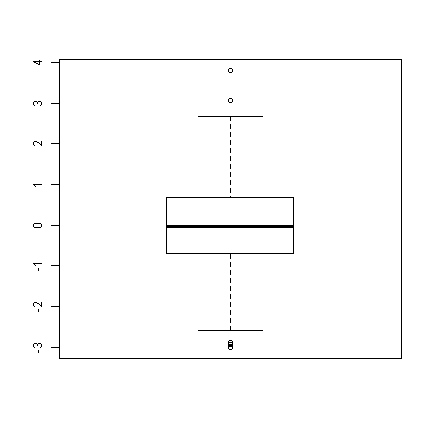
Precise implementations vary, but essentially box plots have a box
with the top being the upper quartile, the bottom being the lower
quartile, a line for the median somehwere inside the box, and
“whiskers” extending the range of the data. R also has the option
to add “notches”, these are based off the interquartile range (IQR)
and are meant to be somewhat like a confidence interval around the
medians. We will work with a simulated data set.
set.seed(1)  # so this is reproducible
## data frame with variable, xn ~N(0, 1)
d <- data.frame(xn = rnorm(1000, mean = 0, sd = 1))

## basic boxplot---looks nice
boxplot(d$xn)
## with the notch
boxplot(d$xn, notch = TRUE)
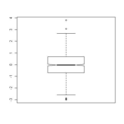
We can see that there are a few “outliers” (the points beyond the
whiskers of the boxplot), but given normal data, it looks very nice.
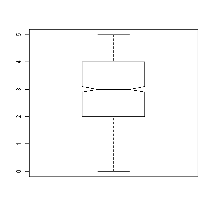
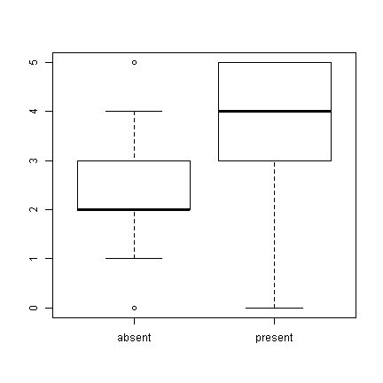
Next we will look at a binomial distribution with 5 trials (like an in class
pop quiz, with 5 true/false questions). We also add a variable, attend, that
indicates whether students attended the last class.
d$attend <- factor(rep(0:1, each = 500), labels = c("absent", "present"))
## set seed to make reproducible and add to boxplot
set.seed(1)
## xb (first 500) ~ B(5, .5) and xb (last 500) ~ B(5, .8)
d$xb <- c(rbinom(500, 5, 0.5), rbinom(500, 5, 0.8))

## notched box plot as before
boxplot(d$xb, notch = TRUE)
## we can also use a formula interface to get separate plots by attendance
boxplot(xb ~ attend, data = d)
Histograms
Box plots are nice and show at least 5 pieces of information for each variable, but
it is not always easy to tell the distribution of a variable from them. To look at
distributions, we can try a histogram. Histograms bin data by counting the number of
observations falling within a certain range, and present the frequency (or probability).
## basic histogram
hist(d$xn)
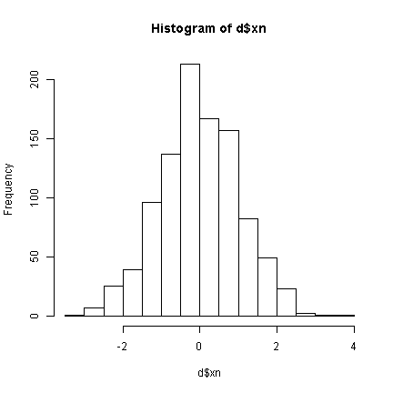
## increase the number of bins (increases resolution)
hist(d$xn, breaks = 25)
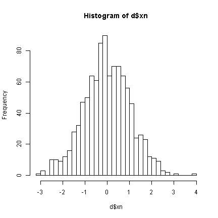
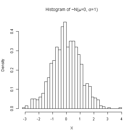
Instead of plotting the frequencies, we can plot the probabilities. We will
also give it better labels. Greek letters (mu and sigma) can be added by placing
them in an expression(). This works for titles, axis labels, and text
directly added to plots.
hist(d$xn, breaks = 25, prob = TRUE, main = expression(paste("Histogram of ~N(",
    mu, "=0, ", sigma, "=1)")), xlab = "X")
## Now examining the 'quiz' data
hist(d$xb, main = "Pop Quiz Results", xlab = "Number Correct")
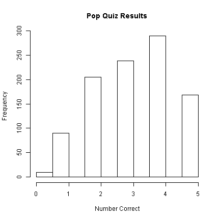
Looking at the histogram, 290 students
got 4/5 questions correct.
Density plots
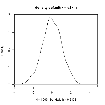
Density plots are great to follow histograms because you can actually plot them right
on top of a histogram if it is of porbabilities instead of frequencies. Density plots
use a smoothing kernel (typically gaussian).
## default density plot
plot(density(d$xn))
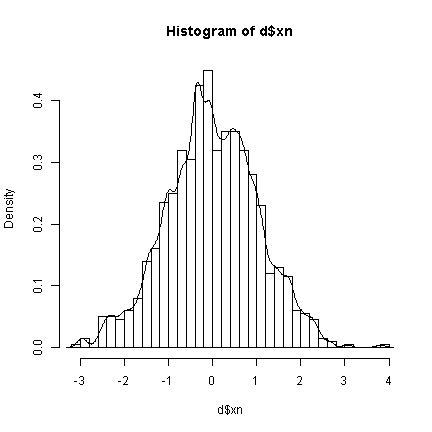
## plot a histogram and add density plot on top setting a smaller
## bandwidth (.1) than before makes it more 'jagged'
hist(d$xn, breaks = 30, prob = TRUE)
lines(density(d$xn, bw = 0.1))
## bandwidth of .4
hist(d$xn, breaks = 30, prob = TRUE)
lines(density(d$xn, bw = 0.4))
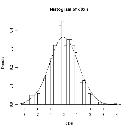
The bandwidths determine the degree of smoothing being done. Higher
bandwidths will be “less true” to the data, but creating smoother density plots.
Next we show the quiz data and also demonstrate the use of the with function,
to avoid having to keep typing the dataset name.
with(d, {
    hist(xb, breaks = 30, prob = TRUE, main = "Histogram of Quiz Scores", xlab = "Number of Questions Correct")
    lines(density(xb, bw = 0.2), lwd = 2, lty = 1)
    lines(density(xb, bw = 1), lwd = 2, lty = 2)
})
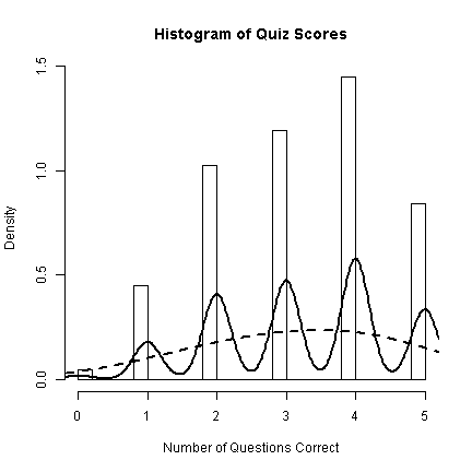
With discrete data like this, the smoothing is not very effective as it
does little to help us understand the data. The trend is better shown with
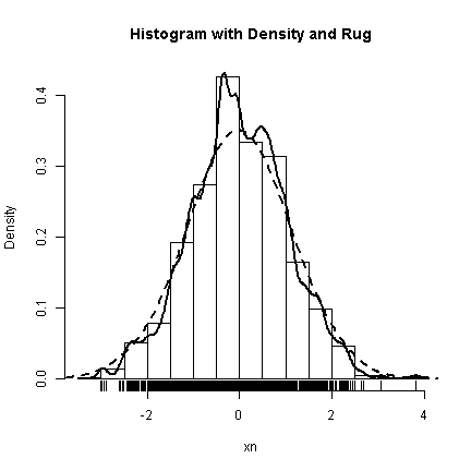
just the bars. To end our demonstrations of graphs for distributions,
we will add a “rug” to the histograms and density plots. The rug is simply a
verticle line for every observation—very true to the data, but imposible to see
multiple observations with the same value. The rug is nice to get insight about
the more rare values in the extremes.
with(d, {
    hist(xn, prob = TRUE, main = "Histogram with Density and Rug")
    lines(density(xn, bw = 0.1), lwd = 2, lty = 1)
    lines(density(xn, bw = 0.5), lwd = 2, lty = 2)
    rug(xn)
})
Plots of functions and complex text
Sometimes it is nice to plot a function directly. Particular for
instructional purposes. Using the curve function in R, you can
plot arbitrary functions evaluated over a range of values, as long as
the function takes a vector, x, and returns a vector the same length as x.
Two common examples in statistics are probability density functions and
cumulative distribution functions. When you are plotting a function,
it also makes sense to show the formula being plotted. This section
shows how to plot functions and how to add complex text (formulae)
to a plot.
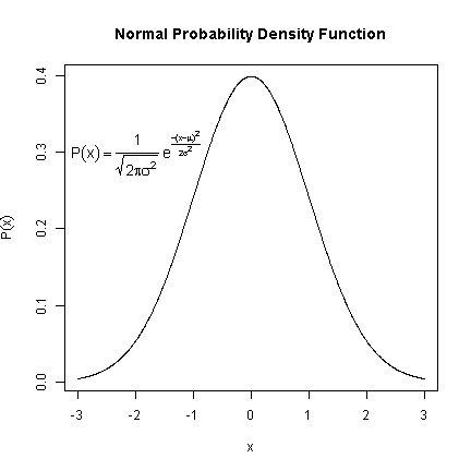
The builtin function dnorm is plotted from -3 to 3. The
interesting part is adding the text. The first argument is
the location on the x axis, the second the location on the y axis.
Next is the text to be plotted. In this case, it is an expression.
Plotting math in R is similar to using LaTeX. frac takes
two arguments, the first is the top of the fraction, the second is
the bottom. Greek letter names are automatically converted to their
symbol form. Finally, the text is made 1.2 times bigger using the
cex (character expansion) argument.
## plot the function from -3 to 3
curve(dnorm, from = -3, to = 3, n = 1000, xlab = "x", ylab = expression(P(x)),
    main = "Normal Probability Density Function")
## add the formula to the plot
text(-2, 0.3, expression(P(x) == paste(frac(1, sqrt(2 * pi * sigma^2)),
    " ", e^{
        frac(-(x - mu)^2, 2 * sigma^2)
    })), cex = 1.2)
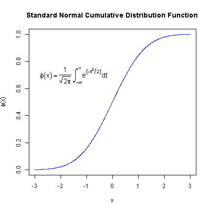
Here is another example where we first define a function
to plot the cumulative percent of normal density of x. This is
used in curve to create the plot. This formula demonstrates
how to add infinity as well as integrals.
## define the function
normCDF <- function(x) {
    x <- dnorm(x)
    cumsum(x)/sum(x)
}
## plot the function from -3 to 3
curve(normCDF, from = -3, to = 3, n = 1000, type = "l", col = "blue",
    xlab = "x", ylab = expression(phi(x)), main = "Standard Normal Cumulative Distribution Function")
## add the formula to the plot
text(-1.5, 0.7, expression(phi(x) == paste(frac(1, sqrt(2 * pi)),
    " ", integral(e^(-t^2/2) * dt, -infinity, x))), cex = 1.2)
Scatter plots
Scatter plots may be the most common way to plot the relationship between two
variables. In R, scatter plots are made using the plot function, which
has a lot of options. We will only scratch the surface now, but you can find out
more from the documentation, ?plot and ?plot.default.
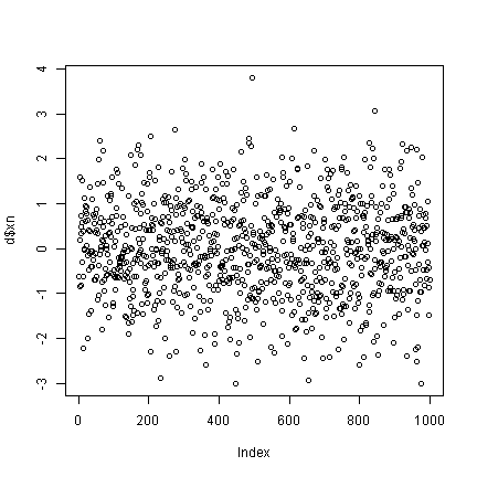
## what happens if you only plot one variable?
plot(d$xn)  # index on the x axis
## create some data correlated with xn
set.seed(2)
d$xnr <- 0.4 * d$xn + rnorm(1000, 0, 1)
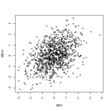
plot(x = d$xn, y = d$xnr)
Up until now, we have not really made too many changes to the default settings.
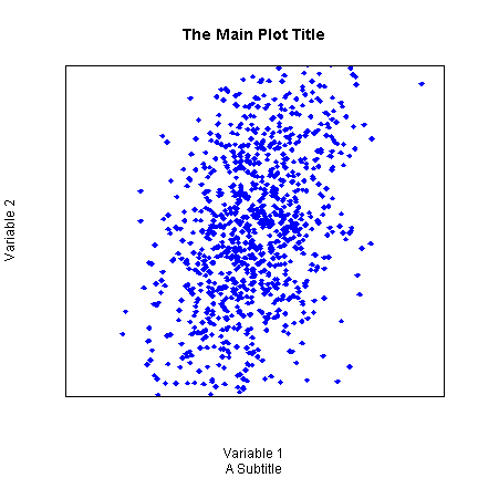
Now we will show many different ways to customize graphs. Although these are
shown for scatter plots, many of the same arguments can be used for other plotting
functions. The pch argument adjusts
the plotting chcharacter. The colour argument
adjusts the point colour. xlimits controls the lower and upper
limit of the X axis (often +/- a twiddle value). xlabel sets
the label for the X axis. xaxt controls the style or turns off
(n) the X axis ticks.
plot(x = d$xn, y = d$xnr, pch = 18, col = "blue", xlim = c(-4, 4),
    ylim = c(-2, 2), xlab = "Variable 1", ylab = "Variable 2", main = "The Main Plot Title",
    sub = "A Subtitle", xaxt = "n", yaxt = "n")
Arguments that accept single values (e.g., pch) also often accept vectors
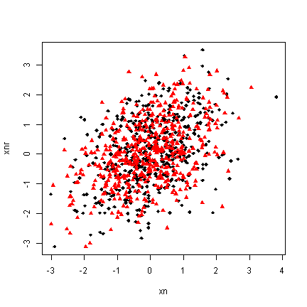
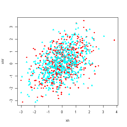
that are the same length as the data. We can take advantage of this to adjust the
plotting character and colour depending on attendance. The trick is to convert the
“absent”, “present” data into numbers for the plotting character and colours. There
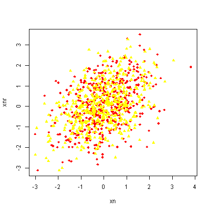
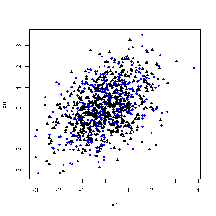
are many ways to accomplish this. ifelse is one way. Attend is a factor and
its levels are automatically used to select two colours (by default black and then red).
We also show how this can be customized in various ways.
## with attend default colour
with(d, plot(x = xn, y = xnr, pch = ifelse(attend == "absent", 18,
    17), col = attend))
## customizing
with(d, plot(x = xn, y = xnr, pch = ifelse(attend == "absent", 18,
    17), col = rainbow(2)[attend]))
## customizing
with(d, plot(x = xn, y = xnr, pch = ifelse(attend == "absent", 18,
    17), col = heat.colors(2)[attend]))
## customizing
with(d, plot(x = xn, y = xnr, pch = ifelse(attend == "absent", 18,
    17), col = ifelse(attend == "absent", "blue", "black")))
Bar plots
Bar plots, are typically information impoverished. They use a lot of space
to present a few values, probably easier to report exactly in a table or in text.
Most often, barplots are anchored at 0, and the height of the bar indicates the mean
of a variable.
## first example
barplot(mean(d$xb), ylab = "Quiz Grade", xlab = "Overall Class")
## mean broken down by attendance
g <- tapply(d$xb, d$attend, FUN = mean)

## now create the bar plot
barplot(g, ylim = c(0, 5))
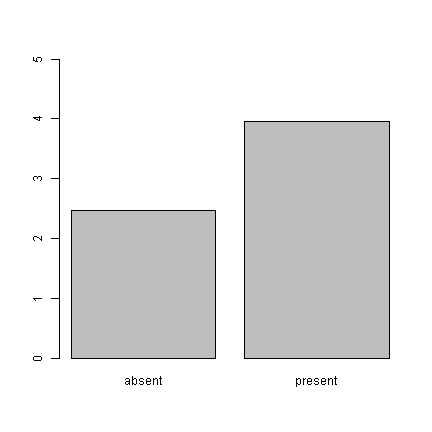
What do these graphs really tell us? Just that the mean of the absent group is
2.47 and the mean of the present group is
3.958. An equivalent presentation would be:
## cex (character expansion) makes the points larger
plot(x = g, pch = 18, cex = 2, ylim = c(0, 5))
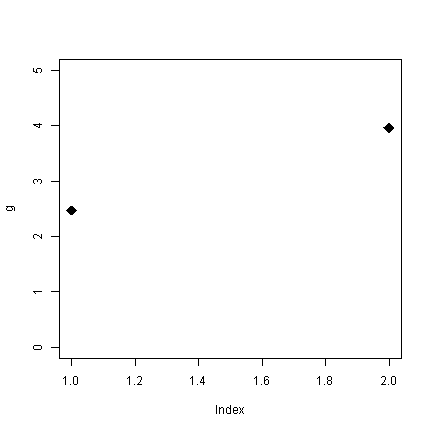
Without all the pointless shading for the bars (remember, only the tops
of the bars convey information), the plot looks sparse. What are the alternatives?
Well, for one, the boxplots we looked at earlier. Alternately, plot the real points
and add the means. Because the outcome is discrete, we use jitter to add a some
noise to get a better sense of the distribution.
with(d, {
    plot(jitter(as.numeric(attend)), xb, xaxt = "n", col = "blue", xlab = "Attendance",
        ylab = "Quiz Score")
    points(x = c(1, 2), y = g, col = "black", pch = 18, cex = 4)
    axis(1, at = c(1, 2), labels = names(g))
})
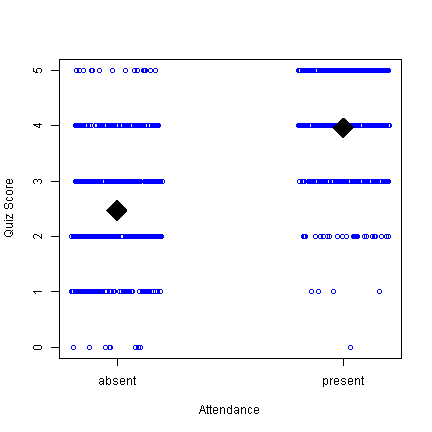
This is probably not the visual display I would choose for these data,
but at least you can see not only the means, but that there are people in the absent
group who score 5 and people in the present that score 0, etc. Along the way, we used
the points function to add points (the means) on top of an existing plot and added
our own X axis to get the labels we wanted.
Piecharts
Pie charts are another problematic type of graph. Why? The human
perceptual system is lousy at accurately quantifying area.
g <- 1:4
names(g) <- letters[1:4]
## How are a, b, c, d growing?
pie(g)
barplot(g)
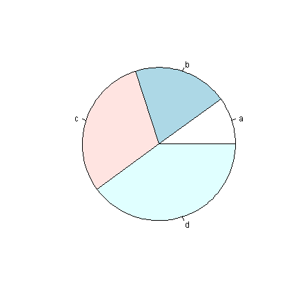
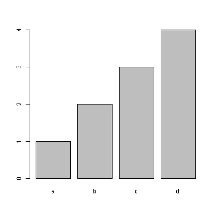
Our visual systems are able to detect small differences in lengths of lines, and
we can quickly see from the bars that the difference between each bar is about equal.
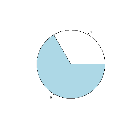
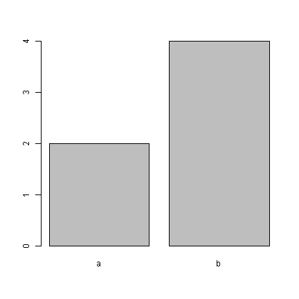
Similarly, in the graphs below, it is easy to tell that “b” is twice as high as “a”, but
difficult to tell “b” has twice the area of “a”.
pie(c(a = 2, b = 4))
barplot(c(a = 2, b = 4))
Summary
We looked at how to make plots in R using boxplot, hist, density,
plot, barplot, pie, as wella s how to customize the colours, shapes,
and labels. We briefly saw how to set our own axes. The next installment of this series
will explore how to really customize plots from tweaking aspects of one plot like adding a
legend to including multiple subplots in one bigger plot.