
Statistical Consulting Seminars: Introduction to SPSS Statistical Computing Seminars
Introduction to SPSS Syntax
NOTE: This seminar was created using SPSS version 21. Some
of the syntax shown below may not work in earlier versions of SPSS.
Here is the link for downloading the syntax file associated with this seminar.
- The SPSS syntax shown in this seminar.
Introduction
The purpose of this seminar is to demonstrate the use of commands that are
useful for managing data in SPSS. Rather than going through each of the
commands in turn and discussing the options available, we are going to focus on
a series of short tasks. Some of these tasks may be similar to things that
you need to do in your work, and other tasks may seem unfamiliar.
Furthermore, we have tried to keep the tasks simple, perhaps too simple, so that
no more than a few commands are needed to accomplish each task. You should
think about different ways that these commands can be combined to do more
complex tasks.
Let’s start by reading in our example dataset. Notice
that this syntax will generate many errors in the output window, but the data
are read into SPSS correctly.
data list list / q1 to q5.
begin data.
3	3	.	.	2
2	2	-9	.	1
3	1	2	.	3
4	1	2       .	-9
-8	1	3	.	2
-8	2	1	.	-9
3	-9	4	.	2
4	4	2	.	3
1	1	1	.	1
2	-9	3	.	2
3	3	2	.	5
3	1	1	.	3
-9	4	4	.	2
.	2	4	.	1
2	3	1	.	4
end data.
dataset name example_data.
missing values q1 to q5 (-8 -9).
Counting the cases in the dataset (unique identifier)
You can create a variable that uniquely identifies each case in your data by
using the system variable $casenum. We also use the formats
command to format all of the variables in our dataset such that they have a
length of 5 and no decimal places. This is done just for esthetics.
compute id = $casenum.
formats q1 to id (f5.0).
exe.
list.
   q1    q2    q3    q4    q5    id

    3     3     .     .     2     1
    2     2    -9     .     1     2
    3     1     2     .     3     3
    4     1     2     .    -9     4
   -8     1     3     .     2     5
   -8     2     1     .    -9     6
    3    -9     4     .     2     7
    4     4     2     .     3     8
    1     1     1     .     1     9
    2    -9     3     .     2    10
    3     3     2     .     5    11
    3     1     1     .     3    12
   -9     4     4     .     2    13
    .     2     4     .     1    14
    2     3     1     .     4    15


Number of cases read:  15    Number of cases listed:  15
Another way to do this is to use the create command with the
csum (cumulative sum) function.
compute id1 = 1.
create id1 = csum(id1).
list.
   q1    q2    q3    q4    q5    id   id1

    3     3     .     .     2     1     1
    2     2    -9     .     1     2     2
    3     1     2     .     3     3     3
    4     1     2     .    -9     4     4
   -8     1     3     .     2     5     5
   -8     2     1     .    -9     6     6
    3    -9     4     .     2     7     7
    4     4     2     .     3     8     8
    1     1     1     .     1     9     9
    2    -9     3     .     2    10    10
    3     3     2     .     5    11    11
    3     1     1     .     3    12    12
   -9     4     4     .     2    13    13
    .     2     4     .     1    14    14
    2     3     1     .     4    15    15

Number of cases read:  15    Number of cases listed:  15
Taking a simple random sample
There are many reasons that you might want to take a simple random sample,
and there are several ways to do it. We will look at several ways to
accomplish this task.
In this example, we create a random variable (called ran_num) using
the uniform function. Next, we sort the cases in our dataset by
this random number.
set seed 156323669.
compute ran_num = uniform(100) + 1.
sort cases by ran_num.
list id ran_num.
   id ran_num

   11    4.26
    2   29.61
    5   34.19
    3   49.33
    7   54.73
    1   55.23
   14   55.50
   10   58.89
    6   60.18
   15   75.17
   13   78.63
    9   88.11
    8   89.81
    4   98.89
   12  100.70

Number of cases read:  15    Number of cases listed:  15
We can now use one of three commands to keep the desired number of cases.
In this example, we will keep 6 cases. When we use the sample
command, we will need to explicitly set the seed before each call to the command
so that our results are reproducible.
temporary.
select if $casenum le 6.
list id ran_num.
    id ran_num

   11    4.26
    2   29.61
    5   34.19
    3   49.33
    7   54.73
    1   55.23

Number of cases read:  6    Number of cases listed:  6
temporary.
n of cases 6.
list id ran_num.
   id ran_num

   11    4.26
    2   29.61
    5   34.19
    3   49.33
    7   54.73
    1   55.23

Number of cases read:  6    Number of cases listed:  6
set seed 822916.
temporary.
sample .4.
list id ran_num.
   id ran_num

    5   34.19
    1   55.23
   14   55.50
   15   75.17
   13   78.63
    9   88.11

Number of cases read:  6    Number of cases listed:  6
set seed 822916.
temporary.
sample 6 from 15.
list id ran_num.
   id ran_num

    5   34.19
    1   55.23
   14   55.50
   15   75.17
   13   78.63
    9   88.11

Number of cases read:  6    Number of cases listed:  6
Notice the difference when you add an execute command before the
list command.
set seed 822916.
temporary.
sample 6 from 15.
exe.
list id ran_num.
   id ran_num

   11    4.26
    2   29.61
    5   34.19
    3   49.33
    7   54.73
    1   55.23
   14   55.50
   10   58.89
    6   60.18
   15   75.17
   13   78.63
    9   88.11
    8   89.81
    4   98.89
   12  100.70

Number of cases read:  15    Number of cases listed:  15
Creating a random identification variable
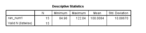
In this example, we will use the rv.normal function to create a
variable with random values. To use this function, you need to specify the
mean and standard deviation.
set seed 1856256.
compute ran_num1 = rv.normal(100, 10).
desc var = ran_num1.
sort cases by ran_num1.
list id ran_num ran_num1.
   id ran_num ran_num1

   11    4.26   84.96
   14   55.50   86.56
    5   34.19   91.00
    4   98.89   92.44
   15   75.17   94.28
    1   55.23   95.85
    7   54.73   96.50
   13   78.63   99.93
    3   49.33  101.80
   10   58.89  102.75
    6   60.18  104.17
    8   89.81  105.59
   12  100.70  107.63
    9   88.11  114.63
    2   29.61  122.04

Number of cases read:  15    Number of cases listed:  15
Numbering groups consecutively
Sometimes you need to make a grouping variable, but you want to be sure that
the values are consecutive. To do this, you can use a scratch variable.
A scratch variable is a temporary variable that will not appear in your active
dataset. It exists only between procedures and is discarded when the new
procedure begins. The name of a scratch variable always starts with #, and
a scratch variable can be either string or numeric. Scratch variables
initialize to 0 for numeric variables and to a null string for string variables.
Also, they are not reinitialized for each case; rather, they keep their current
value when the next case is read. In this sense, they are equivalent to
using the leave command.
Let’s look at a simple example. We will make a new variable called x
that will be the group number (assuming that the values of a are sorted such
that a value of 1 for the variable a indicates a new group).
data list list / a.
begin data.
1
2
3
1
2
3
4
1
2
3
4
5
6
1
2
1
2
3
end data.
dataset name scratch.

compute #x = #x + 1.
if a ne 1 #x = lag(#x).
compute x = #x.
exe.
list.
       a        x

    1.00     1.00
    2.00     1.00
    3.00     1.00
    1.00     2.00
    2.00     2.00
    3.00     2.00
    4.00     2.00
    1.00     3.00
    2.00     3.00
    3.00     3.00
    4.00     3.00
    5.00     3.00
    6.00     3.00
    1.00     4.00
    2.00     4.00
    1.00     5.00
    2.00     5.00
    3.00     5.00

Number of cases read:  18    Number of cases listed:  1
The equivalent syntax using the leave command is below. We will
discuss the leave command shortly.
if a ne lag(a) x1 = 0.
compute x1 = x1 + x.
leave x1.
exe.
list.
Creating an index number
We will start be reading in a new dataset. We will use this dataset
later in the presentation.
data list list / id famid * kidname (A5)  birth age wt * sex (A1).
begin data
1	1	Beth	1	9	60	f
2	1	Bob	2	6	40	m
3	1	Barb	3	3	20	f
4	2	Andy	1	8	80	m
5	2	Al	2	6	50	m
6	2	Ann	3	2	20	f
7	3	Pete	1	6	60	m
8	3	Pam	2	4	40	f
9	3	Phil	3	2	20	m
end data.
dataset name long_to_wide.
list famid kidname age.
 famid kidname    age

  1.00 Beth      9.00
  1.00 Bob       6.00
  1.00 Barb      3.00
  2.00 Andy      8.00
  2.00 Al        6.00
  2.00 Ann       2.00
  3.00 Pete      6.00
  3.00 Pam       4.00
  3.00 Phil      2.00

Number of cases read:  9    Number of cases listed:  9
compute index1 = 1.
if famid = lag(famid) index1 = lag(index1) + 1.
exe.
list famid index1 kidname age.
  famid index1 kidname    age

  1.00   1.00 Beth      9.00
  1.00   2.00 Bob       6.00
  1.00   3.00 Barb      3.00
  2.00   1.00 Andy      8.00
  2.00   2.00 Al        6.00
  2.00   3.00 Ann       2.00
  3.00   1.00 Pete      6.00
  3.00   2.00 Pam       4.00
  3.00   3.00 Phil      2.00

Number of cases read:  9    Number of cases listed:  9
Creating a flag variable for complete cases
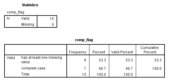
Sometimes it is useful to know how many cases in your dataset have all valid
values, or, in other words, no missing values. You can create a flag
variable, which is a binary variable, that is coded 1 for cases that are
complete and 0 otherwise.
dataset activate example_data.

compute comp_flag = 1.
if missing(q1) or missing(q2) or missing(q3) comp_flag = 0.
value labels comp_flag 0 "has at least one missing value" 1 "complete case" .
exe.
freq var = comp_flag.
list q1 q2 q3 comp_flag.
   q1    q2    q3 comp_flag

    3     3     2     1.00
    .     2     4      .00
   -8     1     3      .00
    4     1     2     1.00
    2     3     1     1.00
    3     3     .      .00
    3    -9     4      .00
   -9     4     4      .00
    3     1     2     1.00
    2    -9     3      .00
   -8     2     1      .00
    4     4     2     1.00
    3     1     1     1.00
    1     1     1     1.00
    2     2    -9      .00

Number of cases read:  15    Number of cases listed:  15
Now we can find out how many valid and missing values each row in the dataset
has. We will use the nvalid and nmissing functions to create
these two new variables.
compute nvalid = nvalid(q1, q2, q3).
compute nmissing = nmissing(q1, q2, q3).
list q1 q2 q3 comp_flag nvalid nmissing.
   q1    q2    q3 comp_flag nvalid nmissing

    3     3     2     1.00    3.00     .00
    .     2     4      .00    2.00    1.00
   -8     1     3      .00    2.00    1.00
    4     1     2     1.00    3.00     .00
    2     3     1     1.00    3.00     .00
    3     3     .      .00    2.00    1.00
    3    -9     4      .00    2.00    1.00
   -9     4     4      .00    2.00    1.00
    3     1     2     1.00    3.00     .00
    2    -9     3      .00    2.00    1.00
   -8     2     1      .00    2.00    1.00
    4     4     2     1.00    3.00     .00
    3     1     1     1.00    3.00     .00
    1     1     1     1.00    3.00     .00
    2     2    -9      .00    2.00    1.00

Number of cases read:  15    Number of cases listed:  15
Finding duplicate pairs
We will use the lag function to help us find duplicate pairs in our
dataset. Let’s assume that we have a group of people, and everyone is
asked to list one friend in the group. Your task is to find all of the
groups of friends, but you realize that if Person A picked Person B, and Person
B picked Person A, you would have the same pair of friends listed twice.
Our task is to find those duplicate pairs.
For this task, we will use an example dataset that has identification
variables that are in string format. We will then make numeric versions of
these variables. We will need both the string and numeric versions to
complete this task. Of course, you could just as easily start with numeric
variables and make string versions of them.
data list list
/ sid1 (A3) sid2 (A3).
begin data.
110 210
514 856
210 110
210 111
693 246
end data.
dataset name duplicates.

recode sid1 (convert) into nid1.
recode sid2 (convert) into nid2.

string pairid (A6).

if (nid1 lt nid2) pairid = concat(sid1, sid2).
if (nid1 gt nid2) pairid = concat(sid2, sid1).

sort cases by pairid.

compute flag = 0.
if pairid = lag(pairid) flag = 1.
value labels flag 0 "not duplicate" 1 "duplicate".
exe.
list.
sid1 sid2   nid1   nid2 pairid   flag

110  210  110.00 210.00 110210    .00
210  110  210.00 110.00 110210   1.00
210  111  210.00 111.00 111210    .00
693  246  693.00 246.00 246693    .00
514  856  514.00 856.00 514856    .00

Number of cases read:  5    Number of cases listed:  5
Comparing datasets
Sometimes you need to compare two datasets, such as when data have been
double-entered. We can use the compare datasets command to do this.
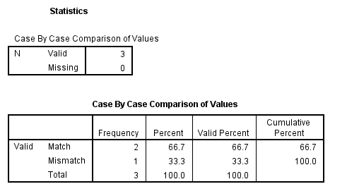
This command was introduced in SPSS version 21. Let’s enter two small
example datasets that have only one difference (in the first row). Note
that both datasets need to be sorted in ascending by variable listed on the
caseid subcommand. A new variable called casescompare will be
added to the active dataset. This new variable can have three values:
-1 means unmatched, 0 means matched and 1 means mismatch.
data list list / id var1 var2 var3.
begin data
1 1 2 3
2 4 5 6
3 7 8 9
end data.
dataset name filea.

data list list / id var1 var2 var3.
begin data
1 1 2 10
2 4 5 6
3 7 8 9
end data.
dataset name fileb.

dataset activate filea.
compare datasets
/compdataset fileb
/variables = all
/caseid id.

freq var = casescompare.
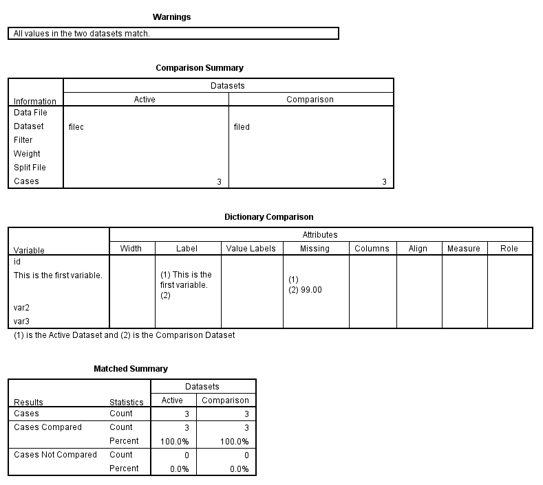
In our next example, we will create two small datasets that have the same
data values but different variable labels.
data list list / id var1 var2 var3.
begin data
1 1 2 3
2 4 5 6
3 7 8 9
end data.
variable labels var1 "This is the first variable.".
dataset name filec.

data list list / id var1 var2 var3.
begin data
1 1 2 3
2 4 5 6
3 7 8 9
end data.
missing values var1 (99).
dataset name filed.

dataset activate filec.
compare datasets
/compdataset filed
/variables = all
/output varproperties = all
/caseid id.
Updating datasets
Sometimes it is necessary to put updated values into a dataset. This
can be done with the update command. This command is not for adding
new variables or new cases (although you can add new cases with this command).
The dataset with the original data is called the master dataset, and the dataset
with the updated values is called the transaction dataset. Both the master
and the transaction datasets must be sorted on the key variable (or variables),
which are listed on the by subcommand. The values in the
transaction dataset will replace those in the master dataset.
data list list / id m1 m2 m3 m4 female.
begin data
1 25 36 41 56 0
2 26 31 49 55 1
3 22 33 44 56 0
4 17 37 41 59 1
5 23 35 48 54 0
6 29 39 41 51 11
end data.
dataset name master.

data list list / id m1 m2 m3 m4 female.
begin data
4 27 37 41 59 1
6 29 39 41 51 1
7 28 32 45 52 0
end data.
dataset name new_updates.

dataset activate master.

update file = *
/file = new_updates
/by id.

list.
    id     m1     m2     m3     m4 female

  1.00  25.00  36.00  41.00  56.00    .00
  2.00  26.00  31.00  49.00  55.00   1.00
  3.00  22.00  33.00  44.00  56.00    .00
  4.00  27.00  37.00  41.00  59.00   1.00
  5.00  23.00  35.00  48.00  54.00    .00
  6.00  29.00  39.00  41.00  51.00   1.00
  7.00  28.00  32.00  45.00  52.00    .00

Number of cases read:  7    Number of cases listed:  7
Creating a level-2 variable
If you have nested data (or data in long form), you may want to create a
level-2 variable. This is a variable that is the mean (or average) of
values within each level 2 unit. Let’s look at an example dataset.
data list list / id score1.
begin data.
1 6
1 2
1 4
2 2
2 2
2 5
3 4
3 5
3 6
4 1
4 2
4 3
end data.
dataset name level2.
list.
    id score1

  1.00   6.00
  1.00   2.00
  1.00   4.00
  2.00   2.00
  2.00   2.00
  2.00   5.00
  3.00   4.00
  3.00   5.00
  3.00   6.00
  4.00   1.00
  4.00   2.00
  4.00   3.00

Number of cases read:  12    Number of cases listed:  12
Now we can use the aggregate command to create our new variable, which
we will call ave_score. First, we need to sort our data by the
variable by which we want to “break” the data. You can think of this as
the grouping variable. The variable (or variables) by which you sort the
data will be listed on the break subcommand. There are many
functions that we can use to create new variables; we are going to use the
mean function.
sort cases id.
aggregate
/break id
/ave_score = mean(score1).
list.
    id score1 ave_score

  1.00   6.00      4.00
  1.00   2.00      4.00
  1.00   4.00      4.00
  2.00   2.00      3.00
  2.00   2.00      3.00
  2.00   5.00      3.00
  3.00   4.00      5.00
  3.00   5.00      5.00
  3.00   6.00      5.00
  4.00   1.00      2.00
  4.00   2.00      2.00
  4.00   3.00      2.00

Number of cases read:  12    Number of cases listed:  12
Collapsing across observations (aggregating data)
Let’s take a closer look at the aggregate command, as it can be very
useful. As we saw in the example above, we can add one (or more) variables
to the active dataset. We can also create a new dataset with the
aggregate command. In this example, we will create a new dataset
called new.sav. This dataset will have only 2 cases because the
variable that we use on the break subcommand, comp_flag, has only
2 values.
dataset activate example_data.
sort cases by comp_flag.
aggregate outfile 'd:datanew.sav'
 /break comp_flag
 /aveq1 = mean(q1).
get file 'd:datanew.sav'.
list.
comp_flag    aveq1

     .00      2.50
    1.00      2.86

Number of cases read:  2    Number of cases listed:  2
Now let’s create multiple new variables in a single call to the aggregate
command, and let’s use some other functions to make these new variables.
We will put the new variables into the active dataset, rather than creating a
new dataset. Some options that are commonly used (but not needed) are
included. We will also include variable labels for each new variable.
Before the aggregate command, we will create a two new variables to use
on the break subcommand. This is done only so that we have a
variable with a few more categories (which may make for a more realistic
example).
dataset activate example_data.
compute gender = 0.
if (mod($casenum, 2) = 1) gender = 1.
compute bvar = 1.
if $casenum gt 5 bvar = 2.
if $casenum gt 9 bvar = 3.
if $casenum gt 12 bvar = 4.
exe.
sort cases by gender bvar.
aggregate outfile = * mode = addvariables
 /break gender bvar
 /sdq1 "standard deviation of q1" = sd(q1)
 /sumq1 "sum of q1" = sum(q1)
 /missq3 "unweighted number of system missing for q3" = numiss(q3)
 /pinq5 "percent of cases between values 2 and 4 for q5" = pin(q5, 2, 4).
list gender bvar q1 sdq1 sumq1 q3 missq3 q5 pinq5.
gender   bvar    q1     sdq1    sumq1    q3  missq3    q5 pinq5

   .00   1.00    -8      .       3.00     3       0     2 100.0
   .00   1.00     3      .       3.00     4       0     2 100.0
   .00   2.00     2      .00     4.00     3       1     2  50.0
   .00   2.00     2      .00     4.00    -9       1     1  50.0
   .00   3.00     4      .71     7.00     2       0    -9 100.0
   .00   3.00     3      .71     7.00     2       0     3 100.0
   .00   4.00     3      .       3.00     1       0     3 100.0
  1.00   1.00     .      .       3.00     4       1     1  66.7
  1.00   1.00     3      .       3.00     .       1     2  66.7
  1.00   1.00    -9      .       3.00     4       1     2  66.7
  1.00   2.00    -8      .       3.00     1       0    -9    .0
  1.00   2.00     3      .       3.00     2       0     5    .0
  1.00   3.00     2      .       2.00     1       0     4 100.0
  1.00   4.00     4     2.12     5.00     2       0     3  50.0
  1.00   4.00     1     2.12     5.00     1       0     1  50.0

Number of cases read:  15    Number of cases listed:  15
The leave command
The leave command “tells” SPSS to leave (or retain) the current value
of the variable as it is, rather than reinitializing it when SPSS reads a new
case. This command also sets the initial value of a case to 0 rather than
system missing (for numeric variables, of course). The leave
command cannot be used with scratch variables. The leave command is
often used to make running (or cumulative) totals and with vectors. We
will see some examples of the use of the leave command with vectors later
in this presentation. As we have already seen, the create command
can also be used to make a cumulative total variable. Because the leave
command does not read the active dataset, it is less resource intensive that the
create command. This may be important if your dataset has millions
of cases.
In the first example, we will make a variable called rtotal that is
the running total of the variable total.
Because we have two groups in our example dataset, our new variable will be the
running total within each group. In the second example, we will make two
new variables. The first variable will be called id, and it will
simply count the number of cases in our example dataset. The variable
cumtotal_leave will be the running total (not broken out by group).
data list list /
group total.
begin data
1 100
1 150
1 125
1 100
2 200
2 250
2 225
2 200
end data.
dataset name leave_group.
sort cases by group.
if group ne lag(group) rtotal = 0.
compute rtotal = rtotal + total.
leave rtotal.
exe.
list.
   group    total   rtotal

    1.00   100.00   100.00
    1.00   150.00   250.00
    1.00   125.00   375.00
    1.00   100.00   475.00
    2.00   200.00   200.00
    2.00   250.00   450.00
    2.00   225.00   675.00
    2.00   200.00   875.00

Number of cases read:  8    Number of cases listed:  8
if missing(lag(total)) id = 0.
leave id.
compute id = id + 1.
if missing(lag(total)) cumtotal_leave = 0.
leave cumtotal_leave.
compute cumtotal_leave = cumtotal_leave + total.
list.
   group    total   rtotal       id cumtotal_leave

    1.00   100.00   100.00     1.00      100.00
    1.00   150.00   250.00     2.00      250.00
    1.00   125.00   375.00     3.00      375.00
    1.00   100.00   475.00     4.00      475.00
    2.00   200.00   200.00     5.00      675.00
    2.00   250.00   450.00     6.00      925.00
    2.00   225.00   675.00     7.00     1150.00
    2.00   200.00   875.00     8.00     1350.00

Number of cases read:  8    Number of cases listed:  8
Review: Three ways to make a running (or cumulative) total
We have seen three ways that you can make a running total variable:
using the create command, using scratch variables, and using the leave
command. Let’s look at these methods side-by-side.
dataset activate leave_group.

create method1 = csum(total).

if missing(lag(total)) #method2 = 0.
compute #method2 = #method2 + total.
compute method2 = #method2.

if missing(lag(total)) method3 = 0.
leave method3.
compute method3 = method3 + total.

list method1 method2 method3.
method1 method2 method3

 100.00  100.00  100.00
 250.00  250.00  250.00
 375.00  375.00  375.00
 475.00  475.00  475.00
 675.00  675.00  675.00
 925.00  925.00  925.00
1150.00  1150.0  1150.0
1350.00  1350.0  1350.0

Number of cases read:  8    Number of cases listed:  8
Do repeat loops
Do repeat loops are very useful for accomplishing repetitive tasks.
In our first example, we are going to make dummy variables (also known as binary
or indicator variables) from a nominal variable. In this example, we will
make dummy variables from the categorical variable race. First, we
will show how this can be done with multiple compute commands.
Next, we show how this can be done with a do repeat loop. As you
can see, if you have many categories, the do repeat loop will save you
lots of typing (and the potential for silly mistakes).
data list free / race.
begin data
1
2
3
4
5
6
.
-9
end data.
missing values race (-9).
dataset name making_indicators.

* make dummies, method 1 .
compute race1=(race=1).
compute race2=(race=2).
compute race3=(race=3).
compute race4=(race=4).
compute race5=(race=5).
compute race6=(race=6).
list.
    race    race1    race2    race3    race4    race5    race6

    1.00     1.00      .00      .00      .00      .00      .00
    2.00      .00     1.00      .00      .00      .00      .00
    3.00      .00      .00     1.00      .00      .00      .00
    4.00      .00      .00      .00     1.00      .00      .00
    5.00      .00      .00      .00      .00     1.00      .00
    6.00      .00      .00      .00      .00      .00     1.00
     .        .        .        .        .        .        .
   -9.00      .        .        .        .        .        .

Number of cases read:  8    Number of cases listed:  8
* make dummies, method 2 .
do repeat a=v1 to v6 /b=1 to 6.
compute a=(race=b).
end repeat.
list.
    race    race1    race2    race3    race4    race5    race6       v1       v2       v3       v4       v5       v6

    1.00     1.00      .00      .00      .00      .00      .00     1.00      .00      .00      .00      .00      .00
    2.00      .00     1.00      .00      .00      .00      .00      .00     1.00      .00      .00      .00      .00
    3.00      .00      .00     1.00      .00      .00      .00      .00      .00     1.00      .00      .00      .00
    4.00      .00      .00      .00     1.00      .00      .00      .00      .00      .00     1.00      .00      .00
    5.00      .00      .00      .00      .00     1.00      .00      .00      .00      .00      .00     1.00      .00
    6.00      .00      .00      .00      .00      .00     1.00      .00      .00      .00      .00      .00     1.00
     .        .        .        .        .        .        .        .        .        .        .        .        .
   -9.00      .        .        .        .        .        .        .        .        .        .        .        .

Number of cases read:  8    Number of cases listed:  8
In our next example, we will recode user-defined missing values to system
missing values.
data list list / var1 var2 var3 var4.
begin data
1 2 3 4
-99 -88 4 5
-77 -99 6 2
5 9 6 8
end data.
dataset name missing.
do repeat v = var1 to var4.
*if v le -77 v = $sysmis.
if any(v, -99, -88, -77) v = $sysmis.
end repeat.
exe.
list.
    var1     var2     var3     var4

    1.00     2.00     3.00     4.00
     .        .       4.00     5.00
     .        .       6.00     2.00
    5.00     9.00     6.00     8.00

Number of cases read:  4    Number of cases listed:  4
In the example below, the values shown on the do repeat command
replace the values in the dataset. The print option on the end
repeat command displays the commands in the log file.
data list list / var1 var3 id var2.
begin data
3 3 3 3
2 2 2 2
end data.
do repeat v=var1 to var2 /val = 1 3 5 7.
compute v = val.
end repeat print.
exe.
list.
    var1     var3       id     var2

    1.00     3.00     5.00     7.00
    1.00     3.00     5.00     7.00

Number of cases read:  2    Number of cases listed:  2
Do if loops
The do if-end if structure is often used for executing multiple
transformations, such as with the compute, recode or count
commands.
The else if command is optional, and it can be repeated as many times
as it is needed. The else command is optional, and it can be used
only once and must follow any else if commands. The end if
command must follow any else if and else commands. You can
have as many nested do if-end if structures as you like, as long your
computer has the memory to support it. Procedures (including graphing
commands) cannot be used in the do if-end if structure. However,
the do if-end if structure can be used to define complex data file
structures (for reading data into SPSS).
When working with do if loops, you need to think carefully about how
control is passed from one command to another. For full details of this,
please see the SPSS Command Syntax Reference Guide in the section on do if-end
if. Basically, control (or the ability to change the value of a variable)
is passed from one command to the next based on the evaluation of the present
command being true, false or missing. If the logical expression is true,
the commands following do if are executed up to the next else if,
else or end if command. Then control passes to the next
command following the end if command. If the expression is false,
control passes to the following else if command. This will continue
until one of the logical expressions is true. As before, the commands
following that logical expression will be executed, and then control will then
pass to the first command after the end if command. If none of the
expressions are true on the do if or any of the else if commands,
the commands following else will be executed. If there is no
else command, the case will not be changed. If all of the conditions
are mutually exclusive, the choice between if and do if is a
matter of preference.
Notice that these two methods of making variable gives different results.
In the do if loop, the first case evaluates as true, so control is not
passed to the else if command; rather, control is passed to the first
command after end if, which is exe. Hence, the value of 1 for the
first case of newvar2 never has a chance to switch to 2, even though the
value of var2 is 1.
data list free / var1 var2.
begin data
1 1
2 1
end data.
if (var1 = 1) newvar1 = 1.
if (var2 = 1) newvar1 = 2.
do if var1 = 1.
compute newvar2 = 1.
else if var2 = 1.
compute newvar2 = 2.
end if.
exe.
list.
    var1     var2  newvar1  newvar2

    1.00     1.00     2.00     1.00
    2.00     1.00     2.00     2.00

Number of cases read:  2    Number of cases listed:  2
You will want to evaluate missing values first, often using the missing
function. This allows the expression to evaluate as either true or false.
If the missing function was used on the else if command, and it
evaluated as true, the compute command immediately following it would not
be executed, because control would have passed to end if.
data list free (",") /a.
begin data
1, , 1,  ,
end data.
dataset name do_if_missing.
compute b = a.
do if missing(b).
compute b1 = 2.
else if b = 1.
compute b1 = 1.
end if.
exe.
list.
       a        b       b1

    1.00     1.00     1.00
     .        .       2.00
    1.00     1.00     1.00
     .        .       2.00

Number of cases read:  4    Number of cases listed:  4
Vectors
A vector is a set of variables that can be referenced by an index number.
The set of variables may already exist in the active dataset, or they may be
created by the vector. The variables in a vector can be numeric or string,
temporary or permanent. The vector itself is temporary and ceases to exist
when the next procedure (or command that causes the dataset to be read) is
encountered. This is one place where extra exe. commands can cause
problems.
Both of the examples below are borrowed from Raynald Levesque’s SPSS
Programming and Data Management, Fourth Edition (pages 143-144). In our
first example, we read in an example dataset and then make two new variables,
called maxvalue and maxcount. Next, we use the vector
command to make a vector called vectorvar which contains the variables
first to fifth. We then loop backwards from 5 to 1 (by -1) to
populate the variable maxcount and to make the variable maxvar.
data list free
/first second third fourth fifth.
begin data
1 2 3 4 5
10 9 8 7 6
1 4 4 4 2
end data.
dataset name vectors.
compute maxvalue = max(first to fifth).
compute maxcount = 0.
list.
 first second  third fourth  fifth maxvalue maxcount

  1.00   2.00   3.00   4.00   5.00    5.00      .00
 10.00   9.00   8.00   7.00   6.00   10.00      .00
  1.00   4.00   4.00   4.00   2.00    4.00      .00

Number of cases read:  3    Number of cases listed:  3
vector vectorvar = first to fifth.
loop #cnt = 5 to 1 by -1.
do if maxvalue = vectorvar(#cnt).
compute maxvar = #cnt.
compute maxcount = maxcount+1.
end if.
end loop.
exe.
list.
 first second  third fourth  fifth maxvalue maxcount maxvar

  1.00   2.00   3.00   4.00   5.00    5.00     1.00    5.00
 10.00   9.00   8.00   7.00   6.00   10.00     1.00    1.00
  1.00   4.00   4.00   4.00   2.00    4.00     3.00    2.00

Number of cases read:  3    Number of cases listed:  3
In our second example, we create some new variables (containing random
values) using a vector. For this example, we must have an active dataset
to which we can add our new variables.
vector vec(4).
loop #cnt = 1 to 4.
compute vec(#cnt) = uniform(1).
end loop.
exe.
list.
 first second  third fourth  fifth maxvalue maxcount maxvar   vec1   vec2   vec3   vec4

  1.00   2.00   3.00   4.00   5.00    5.00     1.00    5.00    .14    .43    .61    .29
 10.00   9.00   8.00   7.00   6.00   10.00     1.00    1.00    .16    .70    .35    .45
  1.00   4.00   4.00   4.00   2.00    4.00     3.00    2.00    .05    .10    .14    .04

Number of cases read:  3    Number of cases listed:  3
Loops
Loops are used to do repeated transformations on the data until a specified
cutoff is reached. There are multiple ways to specify a cutoff. An
unconditional loop will run until it reaches the value specified by mxloops; the
default is 40. This value can be changed using the set mxloops
command. An indexing clause can be used to indicate the starting and
stopping points of the loops. You can also specify the step (the default
is 1). A third option to allow the loop to continue until a specified
condition has been met (similar to the idea of “do while”). You can use
end loop if to specify the ending condition, or you could use the break
command, which is unconditional. This means that the loop will end once
the break command is encountered.
As you might expect, you can nest one loop inside of another. If you do
this, you may want to indent your loops. You can use either + or – as the
character in the first column of the command to keep your syntax compatible with
batch mode processing.
You can also use loops to create a dataset. In the following example,
from pages 152-153 of the Levesque text, we create a casewise dataset from an
aggregated dataset. In the aggregated dataset, there are two females and
two males who are age 20; no one aged 21; one female and four males age 22, etc.
The xsave command is used to save each case to the dataset
tempdata.sav as it is written by the loop. The main difference between
the save command and the xsave command is that the save
command is executed by itself, where as xsave is not executed until data
are read for the next procedure. In this way, xsave reduces
processing time.
data list free / age female male.
begin data
20 2 2
21 0 0
22 1 4
23 3 0
24 0 1
end data.
dataset name loops.
loop #cnt = 1 to sum(female, male).
compute gender = (#cnt > female).
xsave outfile "D:datatempdata.sav"
/keep = age gender.
end loop.
exe.
get file "D:datatempdata.sav".
list.
   age gender

 20.00    .00
 20.00    .00
 20.00   1.00
 20.00   1.00
 22.00    .00
 22.00   1.00
 22.00   1.00
 22.00   1.00
 22.00   1.00
 23.00    .00
 23.00    .00
 23.00    .00
 24.00   1.00

Number of cases read:  13    Number of cases listed:  13
Reshaping data wide to long with the convenience command (varstocases)
In SPSS version 11, two convenience commands were introduced for reshaping
data. One command, varstocases, reshapes data from wide to long
format. The other command, called casestovars, reshapes data from
long to wide format. Of course, you could reshape data in SPSS prior to
version 11, but you had to do manually. In other words, you needed to use
multiple commands in a specific sequence to reshape your data. In this
section, we will show you both the convenience command and the manual method of
reshaping data. It is useful to know how to reshape data manually, because
you may encounter situations in which the convenience command does not meet your
needs. In other words, the manual way of reshaping your data is more
flexible than the convenience commands.
data list list / id trial1 trial2 trial3 female.
begin data
1 16 14 15 0
2 17 19 12 1
3 16 15 19 1
4 17 18 19 0
5 11 12 17 0
6 14 19 18 1
end data.
dataset name wide_data.

varstocases
 /make trial from trial1 to trial3
 /index = number
 /id = id1.
list.
     id1     id female number  trial

       1   1.00    .00     1   16.00
       1   1.00    .00     2   14.00
       1   1.00    .00     3   15.00
       2   2.00   1.00     1   17.00
       2   2.00   1.00     2   19.00
       2   2.00   1.00     3   12.00
       3   3.00   1.00     1   16.00
       3   3.00   1.00     2   15.00
       3   3.00   1.00     3   19.00
       4   4.00    .00     1   17.00
       4   4.00    .00     2   18.00
       4   4.00    .00     3   19.00
       5   5.00    .00     1   11.00
       5   5.00    .00     2   12.00
       5   5.00    .00     3   17.00
       6   6.00   1.00     1   14.00
       6   6.00   1.00     2   19.00
       6   6.00   1.00     3   18.00

Number of cases read:  18    Number of cases listed:  18
Reshaping data wide to long manually (with vectors and loops)
vector Atrial = trial1 to trial3.
loop number = 1 to 3.
compute trial = Atrial(number).
xsave outfile 'd:dataw2lm.sav'
  /drop trial1 trial2 trial3.
end loop.
execute.
get file 'd:dataw2lm.sav'.
list.
    id female number  trial

  1.00    .00   1.00  16.00
  1.00    .00   2.00  14.00
  1.00    .00   3.00  15.00
  2.00   1.00   1.00  17.00
  2.00   1.00   2.00  19.00
  2.00   1.00   3.00  12.00
  3.00   1.00   1.00  16.00
  3.00   1.00   2.00  15.00
  3.00   1.00   3.00  19.00
  4.00    .00   1.00  17.00
  4.00    .00   2.00  18.00
  4.00    .00   3.00  19.00
  5.00    .00   1.00  11.00
  5.00    .00   2.00  12.00
  5.00    .00   3.00  17.00
  6.00   1.00   1.00  14.00
  6.00   1.00   2.00  19.00
  6.00   1.00   3.00  18.00

Number of cases read:  18    Number of cases listed:  18
Reshaping data long to wide with the convenience command (casestovars)
casestovars
/id = id
/index = number.
list.
    id      id1 female trial.1 trial.2 trial.3

  1.00        1    .00   16.00   14.00   15.00
  2.00        2   1.00   17.00   19.00   12.00
  3.00        3   1.00   16.00   15.00   19.00
  4.00        4    .00   17.00   18.00   19.00
  5.00        5    .00   11.00   12.00   17.00
  6.00        6   1.00   14.00   19.00   18.00

Number of cases read:  6    Number of cases listed:  6
Reshaping data wide to long manually (with vectors and the aggregate
command)
sort cases by id number.
vector trial(3).
compute trial(number) = trial.
list id trial trial1 trial2 trial3.

aggregate
 /break id
 /trial1 to trial3 = max(trial1 to trial3).
delete variables trial1 to trial3.
list.
    id female number  trial

  1.00    .00   1.00  16.00
  1.00    .00   2.00  14.00
  1.00    .00   3.00  15.00
  2.00   1.00   1.00  17.00
  2.00   1.00   2.00  19.00
  2.00   1.00   3.00  12.00
  3.00   1.00   1.00  16.00
  3.00   1.00   2.00  15.00
  3.00   1.00   3.00  19.00
  4.00    .00   1.00  17.00
  4.00    .00   2.00  18.00
  4.00    .00   3.00  19.00
  5.00    .00   1.00  11.00
  5.00    .00   2.00  12.00
  5.00    .00   3.00  17.00
  6.00   1.00   1.00  14.00
  6.00   1.00   2.00  19.00
  6.00   1.00   3.00  18.00

Number of cases read:  18    Number of cases listed:  18
Using matrix-end matrix (with OMS)
The example was taken from our SPSS Textbook Examples: Applied Survival
Analysis, Second Edition, Chapter 4 (table 7). Here is a brief description of the task:
We need to get the covariance matrix for the three estimated coefficients. SPSS
does not return the full covariance matrix. Instead, it gives a lower part
of the correlation matrix. We have to compute the full covariance matrix
based on this correlation matrix and the standard errors for the parameter
estimates. This is done making use of both OMS and the matrix language.
oms
/select tables
/if
   subtypes = ['Correlation Matrix of Regression Coefficients']
/destination format = sav
outfile  = 'd:dataasa2corr_table4_7.sav'.
oms
/select tables
/if
   subtypes =  ['Variables in the Equation']
/destination format = sav
outfile  = 'd:dataasa2parms_table4_7.sav'.
coxreg foltime
/method = enter age2 age3 age4
/status folstatus(1)
/print = corr.
omsend.

matrix.
get corr /file="d:dataasa2corr_table4_7.sav"
 /variables=age2 age3
/missing = 0.

compute d=nrow(corr).
compute a = make(d+1, d+1, 0).
loop i = 1 to d.
   loop j = i+1 to d+1.
     compute a(i, j) = corr(j-1, i).
     compute a(j, i) = corr(j-1, i).
   end loop.
end loop.
compute c = ident(d+1) + a.

get se /file="d:dataasa2parms_table4_7.sav"
/variables = se.
compute sigma=mdiag(se).
compute cov = sigma*c*sigma.
print cov.
end matrix.

COV
   .2689919851   .1259938985   .1251235682
   .1259938985   .1983542137   .1260336740
   .1251235682   .1260336740   .1726740755
Using begin program-end program (with Python)
In the example below, we use Python to help us loop through two lists of
variables. SPSS will not allow you to loop through two lists of variables
simultaneously, as you may want to do if you have a list dependent variables and
a list of independent variables. This example was taken from our
SPSS FAQ:
How can I loop through two list of variables? and the full explanation for this
code can be found there.
begin program.
import spss, spssaux
spssaux.OpenDataFile('d:dataelemapi2.sav')
vdict=spssaux.VariableDict()
dlist=vdict.range(start="api00", end="ell")
ilist=vdict.range(start="grad_sch", end="enroll")
ddim = len(dlist)
idim = len(ilist)

if ddim != idim:
     print "The two sequences of variables don't have the same length."
else:
        for i in range(ddim):
             mydvar = dlist[i]
             myivar = ilist[i]

             spss.Submit(r"""
                    regression /dependent %s
                    /method = enter %s.
                                """ %(mydvar, myivar))
end program.