Standard boxplots, as well as a variety of “boxplot like” graphs can be
created using combinations of Stata’s twoway graph commands. If you are trying
to create a relatively standard boxplot, you probably want to use Stata’s
graph box command, however, if you wish to create a boxplot with a
non-standard attribute (e.g. a boxplot that includes a marker at the mean), you
can do this using Stata’s graph twoway commands. The examples below are
based on those shown in the Stata Journal article:
Cox, N.J. (2009). Speaking Stata: Creating and varying box plots. The Stata
Journal, 9(3), 478-496.
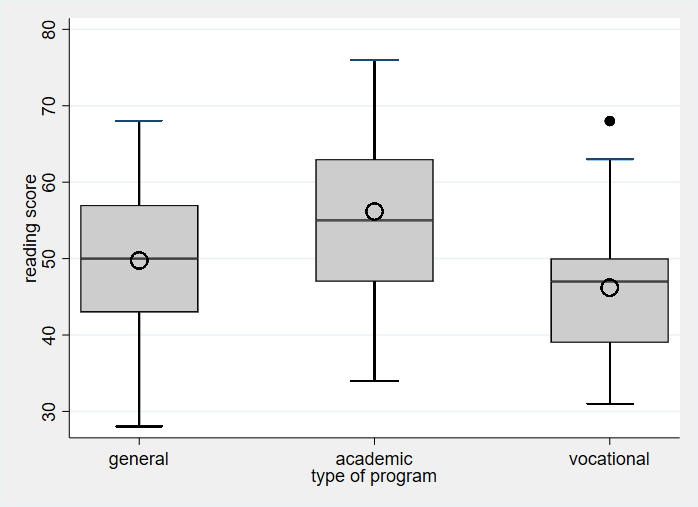
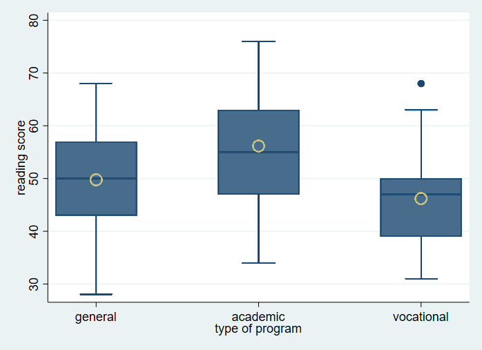
The first example shows how to re-create a boxplot using a twoway graph, as well as how to add a marker at the mean of the distribution.
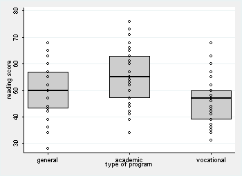
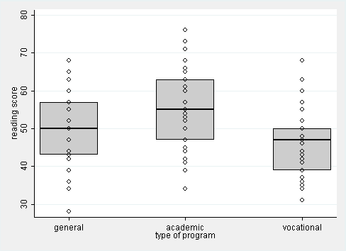
The second example shows how to create a boxplot that displays the individual
data points down the center of the box (instead of whiskers). The examples show the steps of building up the graph to make it easier to understand what is going on.
Example 1: Boxplot by group with a marker for the mean.
Step 1: Data management. Compute all the relevant values (medians, quartiles,
etc.) of read by prog.
use https://stats.idre.ucla.edu/stat/data/hsb2, clear
sort prog

* Use egen to generate the median, quartiles, interquartile range (IQR), and mean.
by prog: egen med = median(read)
by prog: egen lqt = pctile(read), p(25)
by prog: egen uqt = pctile(read), p(75)
by prog: egen iqr = iqr(read)
by prog: egen mean = mean(read)

* Find the lowest value that is more than lqt - 1.5 iqr
* this is used to form the lower "whisker" of the boxplot.
gen l = read if(read >= lqt-1.5*iqr)
by prog: egen ls = min(l)

* Find the highest value that is less than uqt + 1.5 iqr
* this is used to form the upper "whisker" of the boxplot.
gen u = read if(read <= uqt+1.5*iqr)
by prog: egen us = max(u)

* Find any outliers (i.e. values more than 1.5 IQRs from the upper and lower quartiles).
gen outliers = read if(read<=lqt-1.5*iqr | read>=uqt+1.5*iqr)
Step 2: Use rbar to graph the portion of the box below the median.
twoway rbar lqt med prog
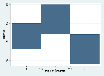
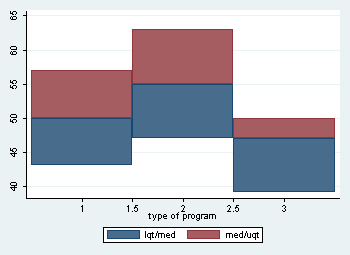
Step3: Add a second rbar command for the portion of the box
above the median.
twoway rbar lqt med prog, || ///
       rbar med uqt prog
Step 4: Use rspike to add the upper and lower “whiskers” and suppress the
display of the legend.
twoway rbar lqt med prog || ///
       rbar med uqt prog || ///
       rspike lqt ls prog || ///
       rspike uqt us prog, legend(off)
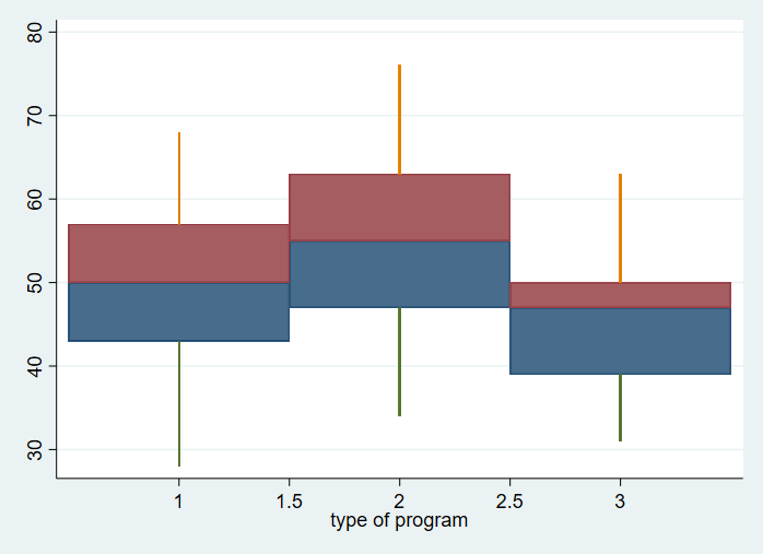
Step 5: Use rcap to add the upper and lower ends to the
whiskers.
twoway rbar lqt med prog || ///
       rbar med uqt prog || ///
       rspike lqt ls prog || ///
       rspike uqt us prog || ///
       rcap ls ls prog, msize(*6)|| ///
       rcap us us prog, msize(*6) legend(off)
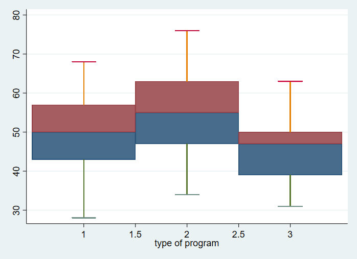
Step 6: Use scatter to show any outliers.
twoway rbar lqt med prog || ///
       rbar med uqt prog || ///
       rspike lqt ls prog || ///
       rspike uqt us prog || ///
       rcap ls ls prog, msize(*6)|| ///
       rcap us us prog, msize(*6) || ///
       scatter outliers prog, legend(off)
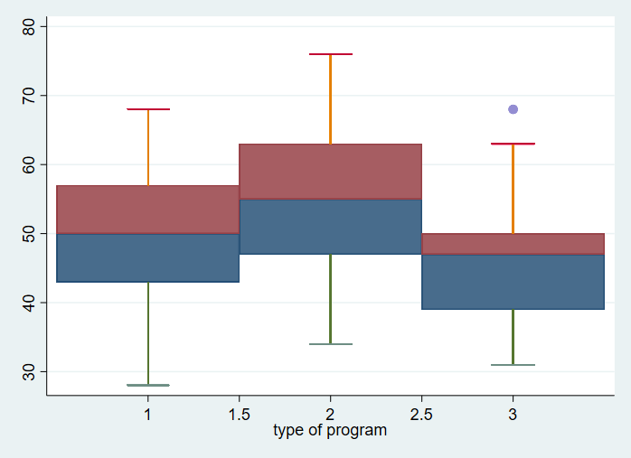
Step 7: Use scatter to place the marker for the mean.
twoway rbar lqt med prog || ///
       rbar med uqt prog || ///
       rspike lqt ls prog || ///
       rspike uqt us prog || ///
       rcap ls ls prog, msize(*6)|| ///
       rcap us us prog, msize(*6) || ///
       scatter outliers prog || ///
       scatter mean prog, msymbol(Oh) msize(*2) legend(off)
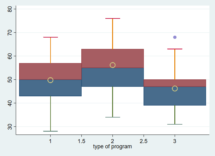
Step 8: Force all of the boxes, lines, etc. to be the same color (pstyle(…)
option), make boxes narrower (barw(#)), and add axis labels.
twoway rbar lqt med prog, pstyle(p1) barw(.5) || ///
       rbar med uqt prog, pstyle(p1) barw(.5) || ///
       rspike lqt ls prog, pstyle(p1) || ///
       rspike uqt us prog, pstyle(p1) || ///
       rcap ls ls prog, msize(*6) pstyle(p1) || ///
       rcap us us prog, msize(*6) pstyle(p1) || ///
       scatter outliers prog, pstyle(p1) || ///
       scatter mean prog, msymbol(Oh) msize(*2) legend(off) ///
       xlabel( 1 "general" 2 "academic" 3 "vocational") ytitle(reading score)
Step 9: Convert to grayscale using the fcolor(…), mcolor(…), and,
lcolor(…) options.
twoway rbar lqt med prog, fcolor(gs12) lcolor(black) barw(.5) || ///
       rbar med uqt prog, fcolor(gs12) lcolor(black) barw(.5) || ///
       rspike lqt ls prog, lcolor(black) || ///
       rspike uqt us prog, lcolor(black) || ///
       rcap ls ls prog, msize(*6) lcolor(black) || ///
       rcap us us prog, msize(*6) pstyle(p1) || ///
       scatter outliers prog, mcolor(black) || ///
       scatter mean prog, msymbol(Oh) msize(*2) fcolor(gs12) mcolor(black) ///
       legend(off)  xlabel( 1 "general" 2 "academic" 3 "vocational") ///
       ytitle(reading score) graphregion(fcolor(gs15))
Example 2: Boxplot by group with datapoints.
Step 1: Use egen to create variables containing the median, upper, and lower
quartiles of read, by prog.
use https://stats.idre.ucla.edu/stat/data/hsb2, clear

sort prog
by prog: egen med = median(read)
by prog: egen lqt = pctile(read), p(25)
by prog: egen uqt = pctile(read), p(75)
Step 2: Use rbar to graph the portion of the box below the median.
twoway rbar lqt med prog
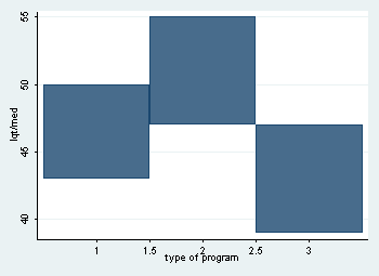
Step 3: Add a second rbar command for the portion of the box above the median.
twoway rbar lqt med prog, || ///
       rbar med uqt prog
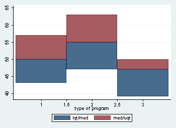
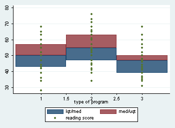
Step 4: Add a scatterplot of read with prog.
twoway rbar lqt med prog, || ///
	rbar med uqt prog || ///
	scatter read prog
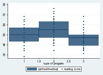
Step 5: Force all portions of the graph to be the same color using pstyle(…).
twoway rbar lqt med prog, pstyle(p1) || ///
	rbar med uqt prog, pstyle(p1) || ///
	scatter read prog, pstyle(p1)
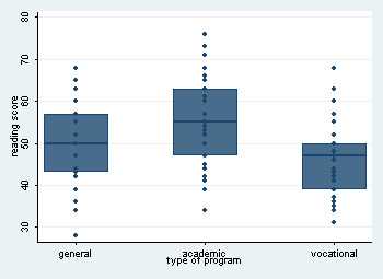
Step 6: Make the boxes narrower using the barw(#) option,
suppress the legend, and add axis labels.
twoway rbar lqt med prog, pstyle(p1) barw(.5) || ///
	rbar med uqt prog, pstyle(p1) barw(.5) || ///
	scatter read prog, pstyle(p1) ///
	legend(off) xlabel( 1 "general" 2 "academic" 3 "vocational") ///
	ytitle(reading score)
Step 7: Convert to gray scale using fcolor(…), lcolor(…),
and mcolor(…) if desired.
twoway rbar lqt med prog, barw(.5) fcolor(gs12) lcolor(black) || ///
	rbar med uqt prog, barw(.5) fcolor(gs12) lcolor(black) || ///
	scatter read prog, graphregion(fcolor(gs15)) mcolor(black) msymbol(Oh) ///
	legend(off) xlabel( 1 "general" 2 "academic" 3 "vocational") ///
	ytitle(reading score)