
Version info: Code for this page was tested in Stata 12.
Multinomial logistic regression is used to model nominal
outcome variables, in which the log odds of the outcomes are modeled as a linear
combination of the predictor variables.
Please note: The purpose of this page is to show how to use various data analysis commands.
It does not cover all aspects of the research process which researchers are expected to do. In
particular, it does not cover data cleaning and checking, verification of assumptions, model
diagnostics and potential follow-up analyses.
Examples of multinomial logistic regression
Example 1. People’s occupational choices might be influenced
by their parents’ occupations and their own education level. We can study the
relationship of one’s occupation choice with education level and father’s
occupation. The occupational choices will be the outcome variable which
consists of categories of occupations.
Example 2. A biologist may be
interested in food choices that alligators make. Adult alligators might have
different preferences from young ones. The outcome variable here will be the
types of food, and the predictor variables might be size of the alligators
and other environmental variables.
Example 3. Entering high school students make program choices among general program,
vocational program and academic program. Their choice might be modeled using
their writing score and their social economic status.
Description of the data
For our data analysis example, we will expand the third example using the
hsbdemo data set. Let’s first read in the data.
use https://stats.idre.ucla.edu/stat/data/hsbdemo, clear
The data set contains variables on 200 students. The outcome variable is prog, program type. The predictor variables
are social economic status, ses, a three-level categorical variable
and writing score, write, a continuous variable. Let’s start with
getting some descriptive statistics of the
variables of interest.
tab prog ses, chi2

   type of |               ses
   program |       low     middle       high |     Total
-----------+---------------------------------+----------
   general |        16         20          9 |        45
  academic |        19         44         42 |       105
  vocation |        12         31          7 |        50
-----------+---------------------------------+----------
     Total |        47         95         58 |       200

          Pearson chi2(4) =  16.6044   Pr = 0.002
table prog, con(mean write sd write) ------------------------------------ type of | program | mean(write) sd(write) ----------+------------------------- general | 51.33333 9.397776 academic | 56.25714 7.943343 vocation | 46.76 9.318754 ------------------------------------
Analysis methods you might consider
- Multinomial logistic regression: the focus of this page.
- Multinomial probit regression: similar to multinomial logistic
regression but with independent normal error terms. - Multiple-group discriminant function analysis: A multivariate method for
multinomial outcome variables - Multiple logistic regression analyses, one for each pair of outcomes:
One problem with this approach is that each analysis is potentially run on a different
sample. The other problem is that without constraining the logistic models,
we can end up with the probability of choosing all possible outcome categories
greater than 1. - Collapsing number of categories to two and then doing a logistic regression: This approach
suffers from loss of information and changes the original research questions to
very different ones. - Ordinal logistic regression: If the outcome variable is truly ordered
and if it also satisfies the assumption of proportional
odds, then switching to ordinal logistic regression will make the model more
parsimonious. - Alternative-specific multinomial probit regression: allows
different error structures therefore allows to relax the independence of
irrelevant alternatives (IIA, see below “Things to Consider”) assumption.
This requires that the data structure be choice-specific. - Nested logit model: also relaxes the IIA assumption, also
requires the data structure be choice-specific.
Multinomial logistic regression
Below we use the mlogit command to estimate a multinomial logistic regression
model. The i. before ses indicates that ses is a indicator
variable (i.e.,
categorical variable), and that it should be included in the model. We
have also used the option “base” to indicate the category we would want
to use for the baseline comparison group. In the model below, we have chosen to
use the academic program type as the baseline category.
 mlogit prog i.ses write, base(2)

Iteration 0:   log likelihood = -204.09667
Iteration 1:   log likelihood = -180.80105
Iteration 2:   log likelihood = -179.98724
Iteration 3:   log likelihood = -179.98173
Iteration 4:   log likelihood = -179.98173

Multinomial logistic regression                   Number of obs   =        200
                                                  LR chi2(6)      =      48.23
                                                  Prob > chi2     =     0.0000
Log likelihood = -179.98173                       Pseudo R2       =     0.1182

------------------------------------------------------------------------------
        prog |      Coef.   Std. Err.      z    P>|z|     [95% Conf. Interval]
-------------+----------------------------------------------------------------
general      |
         ses |
          2  |   -.533291   .4437321    -1.20   0.229     -1.40299     .336408
          3  |  -1.162832   .5142195    -2.26   0.024    -2.170684   -.1549804
             |
       write |  -.0579284   .0214109    -2.71   0.007    -.0998931   -.0159637
       _cons |   2.852186   1.166439     2.45   0.014     .5660075    5.138365
-------------+----------------------------------------------------------------
academic     |  (base outcome)
-------------+----------------------------------------------------------------
vocation     |
         ses |
          2  |   .2913931   .4763737     0.61   0.541    -.6422822    1.225068
          3  |  -.9826703   .5955669    -1.65   0.099     -2.14996    .1846195
             |
       write |  -.1136026   .0222199    -5.11   0.000    -.1571528   -.0700524
       _cons |     5.2182   1.163549     4.48   0.000     2.937686    7.498714
------------------------------------------------------------------------------
- In the output above, we first see the iteration log, indicating how quickly
the model converged. The log likelihood (-179.98173) can be usedin comparisons of nested models, but we won’t show an example of comparing
models here - The likelihood ratio chi-square of48.23 with a p-value < 0.0001 tells us that our model as a whole fits
significantly better than an empty model (i.e., a model with no
predictors) - The output above has two parts, labeled with the categories of the
outcome variable prog. They correspond to the two equations below:$$ln\left(\frac{P(prog=general)}{P(prog=academic)}\right) = b_{10} + b_{11}(ses=2) + b_{12}(ses=3) + b_{13}write$$
$$ln\left(\frac{P(prog=vocation)}{P(prog=academic)}\right) = b_{20} + b_{21}(ses=2) + b_{22}(ses=3) + b_{23}write$$
where \(b\)’s are the regression coefficients.
- A one-unit increase in the variable write is associated with a
.058 decrease in the relative log odds of being in general program vs.
academic program . - A one-unit increase in the variable write is associated with a
.1136 decrease in the relative log odds of being in vocation program vs.
academic program. - The relative log odds of being in general program vs. in academic program will
decrease by 1.163 if moving from the lowest level of ses (ses==1) to the
highest level of ses (ses==3).
- A one-unit increase in the variable write is associated with a
The ratio of the probability of choosing one outcome category over the
probability of choosing the baseline category is often referred to as relative risk
(and it is also sometimes referred to as odds as we have just used to described the
regression parameters above). Relative risk can be obtained by
exponentiating the linear equations above, yielding
regression coefficients that are relative risk ratios for a unit change in the
predictor variable. We can use the rrr option for
mlogit command to display the regression results in terms of relative risk
ratios.
mlogit, rrr

Multinomial logistic regression                   Number of obs   =        200
                                                  LR chi2(6)      =      48.23
                                                  Prob > chi2     =     0.0000
Log likelihood = -179.98173                       Pseudo R2       =     0.1182

------------------------------------------------------------------------------
        prog |        RRR   Std. Err.      z    P>|z|     [95% Conf. Interval]
-------------+----------------------------------------------------------------
general      |
         ses |
          2  |    .586671   .2603248    -1.20   0.229     .2458607     1.39991
          3  |   .3125996   .1607448    -2.26   0.024     .1140996     .856432
             |
       write |   .9437175   .0202059    -2.71   0.007     .9049342     .984163
       _cons |   17.32562   20.20928     2.45   0.014     1.761221    170.4369
-------------+----------------------------------------------------------------
academic     |  (base outcome)
-------------+----------------------------------------------------------------
vocation     |
         ses |
          2  |   1.338291   .6375264     0.61   0.541     .5260904    3.404399
          3  |   .3743103   .2229268    -1.65   0.099     .1164888    1.202761
             |
       write |   .8926126   .0198338    -5.11   0.000     .8545734    .9323449
       _cons |   184.6016    214.793     4.48   0.000     18.87213    1805.719
------------------------------------------------------------------------------
- The relative risk ratio for a one-unit increase in the variable write is
.9437 (exp(-.0579284) from the output of the first mlogit command
above) for being in general program vs. academic program. - The relative risk ratio switching from ses = 1 to 3 is .3126 for being
in general program vs. academic program. In other words, the expected risk
of staying in the general program is lower for subjects who are high in
ses.
We can test for an overall effect of ses
using the test command. Below we see that the overall effect of ses is
statistically significant.
test 2.ses 3.ses

 ( 1)  [general]2.ses = 0
 ( 2)  [academic]2.ses = 0
 ( 3)  [vocation]2.ses = 0
 ( 4)  [general]3.ses = 0
 ( 5)  [academic]3.ses = 0
 ( 6)  [vocation]3.ses = 0
       Constraint 2 dropped
       Constraint 5 dropped

           chi2(  4) =   10.82
         Prob > chi2 =    0.0287
More specifically, we can also test if the effect of 3.ses in
predicting general vs. academic equals the effect of 3.ses in
predicting vocation vs. academic using the test command again. The test
shows that the effects are not statistically different from each other.
test [general]3.ses = [vocation]3.ses

 ( 1)  [general]3.ses - [vocation]3.ses = 0

           chi2(  1) =    0.08
         Prob > chi2 =    0.7811
You can also use predicted probabilities to help you understand the model.
You can calculate predicted probabilities using the margins command. Below we use the margins command to
calculate the predicted probability of choosing each program type at each level
of ses, holding all other variables in the model at their means. Since
there are three possible outcomes, we will need to use the margins command three
times, one for each outcome value.
margins ses, atmeans predict(outcome(1))

Adjusted predictions                              Number of obs   =        200
Model VCE    : OIM

Expression   : Pr(prog==general), predict(outcome(1))
at           : 1.ses           =        .235 (mean)
               2.ses           =        .475 (mean)
               3.ses           =         .29 (mean)
               write           =      52.775 (mean)

------------------------------------------------------------------------------
             |            Delta-method
             |     Margin   Std. Err.      z    P>|z|     [95% Conf. Interval]
-------------+----------------------------------------------------------------
         ses |
          1  |   .3581927   .0726423     4.93   0.000     .2158163     .500569
          2  |   .2283338   .0451162     5.06   0.000     .1399075      .31676
          3  |   .1784932   .0540486     3.30   0.001     .0725598    .2844266
------------------------------------------------------------------------------

margins ses, atmeans predict(outcome(2))

Adjusted predictions                              Number of obs   =        200
Model VCE    : OIM

Expression   : Pr(prog==academic), predict(outcome(2))
at           : 1.ses           =        .235 (mean)
               2.ses           =        .475 (mean)
               3.ses           =         .29 (mean)
               write           =      52.775 (mean)

------------------------------------------------------------------------------
             |            Delta-method
             |     Margin   Std. Err.      z    P>|z|     [95% Conf. Interval]
-------------+----------------------------------------------------------------
         ses |
          1  |   .4396842   .0779925     5.64   0.000     .2868217    .5925466
          2  |   .4777488   .0552593     8.65   0.000     .3694426     .586055
          3  |   .7009021   .0663042    10.57   0.000     .5709483    .8308559
------------------------------------------------------------------------------

margins ses, atmeans predict(outcome(3))

Adjusted predictions                              Number of obs   =        200
Model VCE    : OIM

Expression   : Pr(prog==vocation), predict(outcome(3))
at           : 1.ses           =        .235 (mean)
               2.ses           =        .475 (mean)
               3.ses           =         .29 (mean)
               write           =      52.775 (mean)

------------------------------------------------------------------------------
             |            Delta-method
             |     Margin   Std. Err.      z    P>|z|     [95% Conf. Interval]
-------------+----------------------------------------------------------------
         ses |
          1  |   .2021232   .0599647     3.37   0.001     .0845945    .3196519
          2  |   .2939174   .0503617     5.84   0.000     .1952103    .3926246
          3  |   .1206047     .04643     2.60   0.009     .0296037    .2116058
------------------------------------------------------------------------------
We can use the marginsplot command to plot predicted
probabilities by ses for each category of prog. Plots created
by marginsplot are based on the last margins command
run. Furthermore, we can combine the three marginsplots into one
graph to facilitate comparison using the graph combine
command. As it is generated, each marginsplot must be given a name,
which will be used by graph combine. Additionally, we would
like the y-axes to have the same range, so we use the ycommon
option with graph combine .
margins ses, atmeans predict(outcome(1))
marginsplot, name(general)
margins ses, atmeans predict(outcome(2))
marginsplot, name(academic)
margins ses, atmeans predict(outcome(3))
marginsplot, name(vocational)
graph combine general academic vocational, ycommon

Another way to understand the model using the predicted probabilities is to
look at the averaged predicted probabilities for different values of the
continuous predictor variable write, averaging across levels of ses.
margins, at(write = (30(10) 70)) predict(outcome(1)) vsquish

Predictive margins                                Number of obs   =        200
Model VCE    : OIM

Expression   : Pr(prog==general), predict(outcome(1))
1._at        : write           =          30
2._at        : write           =          40
3._at        : write           =          50
4._at        : write           =          60
5._at        : write           =          70

------------------------------------------------------------------------------
             |            Delta-method
             |     Margin   Std. Err.      z    P>|z|     [95% Conf. Interval]
-------------+----------------------------------------------------------------
         _at |
          1  |   .2130954   .0774327     2.75   0.006     .0613302    .3648606
          2  |   .2569932   .0529761     4.85   0.000     .1531619    .3608245
          3  |   .2543008   .0336297     7.56   0.000     .1883878    .3202138
          4  |   .2057855   .0371536     5.54   0.000     .1329658    .2786052
          5  |   .1423089   .0481683     2.95   0.003     .0479007    .2367172
------------------------------------------------------------------------------

margins, at(write = (30(10) 70)) predict(outcome(2)) vsquish

Predictive margins                                Number of obs   =        200
Model VCE    : OIM

Expression   : Pr(prog==academic), predict(outcome(2))
1._at        : write           =          30
2._at        : write           =          40
3._at        : write           =          50
4._at        : write           =          60
5._at        : write           =          70

------------------------------------------------------------------------------
             |            Delta-method
             |     Margin   Std. Err.      z    P>|z|     [95% Conf. Interval]
-------------+----------------------------------------------------------------
         _at |
          1  |   .1348408   .0525979     2.56   0.010     .0317507    .2379308
          2  |   .2808143   .0553213     5.08   0.000     .1723867     .389242
          3  |   .4773283   .0397591    12.01   0.000      .399402    .5552547
          4  |   .6680752   .0434689    15.37   0.000     .5828776    .7532727
          5  |   .8075124   .0545504    14.80   0.000     .7005956    .9144291
------------------------------------------------------------------------------

margins, at(write = (30(10) 70)) predict(outcome(3)) vsquish

Predictive margins                                Number of obs   =        200
Model VCE    : OIM

Expression   : Pr(prog==vocation), predict(outcome(3))
1._at        : write           =          30
2._at        : write           =          40
3._at        : write           =          50
4._at        : write           =          60
5._at        : write           =          70

------------------------------------------------------------------------------
             |            Delta-method
             |     Margin   Std. Err.      z    P>|z|     [95% Conf. Interval]
-------------+----------------------------------------------------------------
         _at |
          1  |   .6520638   .0944041     6.91   0.000     .4670353    .8370924
          2  |   .4621925   .0614388     7.52   0.000     .3417747    .5826102
          3  |   .2683708   .0342932     7.83   0.000     .2011575    .3355842
          4  |   .1261393     .03019     4.18   0.000     .0669679    .1853107
          5  |   .0501787   .0216863     2.31   0.021     .0076744     .092683
------------------------------------------------------------------------------
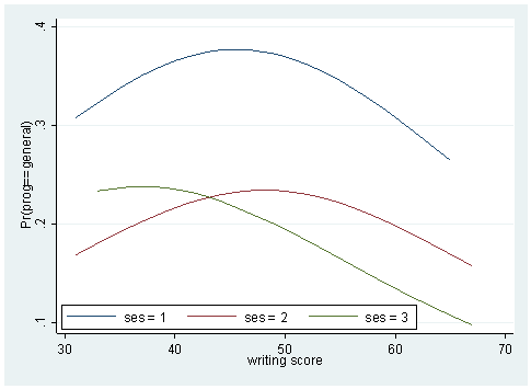
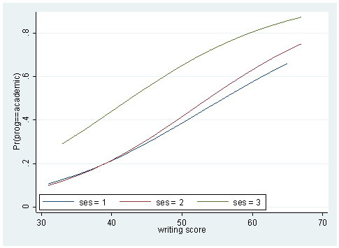
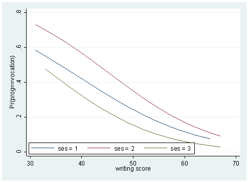
Sometimes, a couple of plots can convey a good deal amount of information.
Below, we plot the predicted probabilities against the writing score by the
level of ses for different levels of the outcome variable.
predict p1 p2 p3
sort write
twoway (line p1 write if ses ==1) (line p1 write if ses==2) (line p1 write if ses ==3), ///
	legend(order(1 "ses = 1" 2 "ses = 2" 3 "ses = 3") ring(0) position(7) row(1))
twoway (line p2 write if ses ==1) (line p2 write if ses==2) (line p2 write if ses ==3), ///
        legend(order(1 "ses = 1" 2 "ses = 2" 3 "ses = 3") ring(0) position(7) row(1))
twoway (line p3 write if ses ==1) (line p3 write if ses==2) (line p3 write if ses ==3), ///
	legend(order(1 "ses = 1" 2 "ses = 2" 3 "ses = 3") ring(0) position(7) row(1))
We may also wish to see measures of how well our model fits. This can be particularly useful when comparing
competing models. The user-written command fitstat produces a
variety of fit statistics. You can find more information on fitstat and
download the program by using command
search fitstat in Stata (see
How can I use the search command to search for programs and get additional help?
for more information about using search).
fitstat

Measures of Fit for mlogit of prog
fit
Log-Lik Intercept Only:       -204.097   Log-Lik Full Model:           -179.982
D(185):                        359.963   LR(6):                          48.230
                                         Prob > LR:                       0.000
McFadden's R2:                   0.118   McFadden's Adj R2:               0.045
ML (Cox-Snell) R2:               0.214   Cragg-Uhler(Nagelkerke) R2:      0.246
Count R2:                        0.610   Adj Count R2:                    0.179
AIC:                             1.950   AIC*n:                         389.963
BIC:                          -620.225   BIC':                          -16.440
BIC used by Stata:             402.350   AIC used by Stata:             375.963
Things to consider
- The Independence of Irrelevant Alternatives (IIA) assumption: roughly,
the IIA assumption means that adding or deleting alternative outcome
categories does not affect the odds among the remaining outcomes. Test of
the IIA assumption can be performed
by using the Stata command mlogtest, iia. However, as of
April 23, 2010, mlogtest, iia does not work with factor variables. There are alternative modeling methods
that relax the IIA assumption,
such as alternative-specific multinomial probit models or nested logit
models. - Diagnostics and model fit: unlike logistic regression where there are
many statistics for performing model diagnostics, it is not as
straightforward to do diagnostics with multinomial logistic regression
models. Model fit statistics can be obtained via the fitstat command.
For the purpose of detecting outliers or influential data points, one can
run separate logit models and use the diagnostics tools on each model. - Pseudo-R-Squared: the R-squared offered in the output is basically the
change in terms of log-likelihood from the intercept-only model to the
current model. It does not convey the same information as the R-square for
linear regression, even though it is still “the higher, the better”. - Sample size: multinomial regression uses a maximum likelihood estimation
method, it requires a large sample size. It also uses multiple
equations. This implies that it requires an even larger sample size than ordinal or
binary logistic regression. - Complete or quasi-complete separation: Complete separation implies that
the outcome variable separates a predictor variable completely, leading
to perfect prediction by the predictor variable. Unlike running a logit model,
Stata does not offer a warning when this happens. Instead it continues to
compute iteratively and requires a manual quit to stop the process. Perfect prediction means that only one value of a predictor
variable is associated with only one value of the response variable. But you can tell from the output of the
regression coefficients that something is wrong. You can then do a two-way tabulation of the outcome
variable with the problematic variable to confirm this and then rerun the model
without the problematic variable. - Empty cells or small cells: You should check for empty or small
cells by doing a cross-tabulation between categorical predictors and
the outcome variable. If a cell has very few cases (a small cell), the
model may become unstable or it might not even run at all. - Perhaps your data may not perfectly meet the assumptions and your
standard errors might be off the mark. You might wish to see our page that
shows alternative methods for computing standard
errors that Stata offers. - Sometimes observations are clustered into groups (e.g., people within
families, students within classrooms). In such cases, you may want to see
our page on non-independence within clusters.
See also
References
- Long, J. S. and Freese, J. (2006)
Regression Models for Categorical and Limited Dependent Variables Using Stata,
Second Edition. College Station, Texas: Stata Press. - Hosmer, D. and Lemeshow, S. (2000) Applied Logistic Regression (Second
Edition). New York: John Wiley & Sons, Inc.. - Agresti, A. (1996) An Introduction to Categorical Data
Analysis. New York: John Wiley & Sons, Inc.