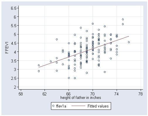
Figure 6.1, page 87.
NOTE: Throughout this chapter and the next, the variables FFEV1 and MFEV1 have been divided by
100 before use in analyses. We have named these modified variables FFEV1a and MFEV1a,
respectively.
NOTE: To get the regression line on the graph, you need to run the
regression and get the predicted values. Those values are included on the
plot and are connected by the line.
use https://stats.idre.ucla.edu/stat/stata/examples/cama4/lung, clear

generate ffev1a = ffev1/100
regress ffev1a fheight
graph twoway (scatter ffev1a fheight, msymbol(Oh)) (lfit  ffev1a fheight), ///
	xlabel(58 62 to 78, grid) ylabel(2 2.5 to 6.5, angle(0)) ///
	ytitle(FFEV1)
Page 88. The descriptive statistics at the top of the page.
summarize ffev1a fheight

    Variable |     Obs        Mean   Std. Dev.       Min        Max
-------------+-----------------------------------------------------
      ffev1a |     150    4.093267   .6507523        2.5       5.85
     fheight |     150       69.26   2.779189         61         76
Page 98. The correlation in the middle of the page.
correlate fheight ffev1a
(obs=150)

             |  fheight   ffev1a
-------------+------------------
     fheight |   1.0000
      ffev1a |   0.5044   1.0000
Table 6.2, page 100.
NOTE: We need to generate the residuals for use in the next figure.
regress ffev1a fheight
predict resid, resid

      Source |       SS       df       MS              Number of obs =     150
-------------+------------------------------           F(  1,   148) =   50.50
       Model |  16.0531702     1  16.0531702           Prob > F      =  0.0000
    Residual |  47.0451258   148  .317872472           R-squared     =  0.2544
-------------+------------------------------           Adj R-squared =  0.2494
       Total |   63.098296   149  .423478497           Root MSE      =   .5638

------------------------------------------------------------------------------
      ffev1a |      Coef.   Std. Err.      t    P>|t|     [95% Conf. Interval]
-------------+----------------------------------------------------------------
     fheight |   .1181052   .0166194     7.11   0.000     .0852633    .1509472
       _cons |  -4.086702   1.151979    -3.55   0.001    -6.363155    -1.81025
------------------------------------------------------------------------------
Figure 6.10, page 112. This has been skipped for now.
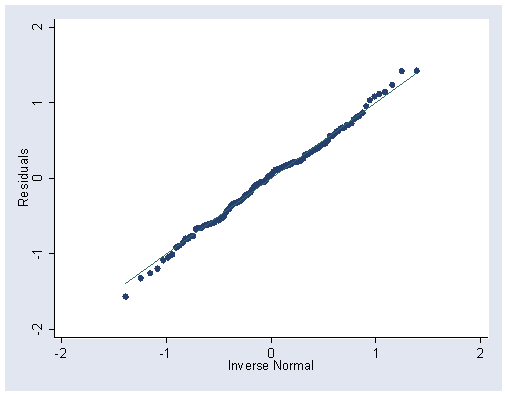
Figure 6.12, page 116.
NOTE: The graph produced by the qnorm command in Stata has the axes reversed from that
shown in the text.
qnorm resid