
Part of table 12.1, page 323. The variable index corresponds to the row value in table 12.1.
use https://stats.idre.ucla.edu/stat/stata/examples/chp/p323, clear

generate index = _n
list in f/5

            y         x1         x2         x3      index
  1.        0      -62.8      -89.5        1.7          1
  2.        0        3.3       -3.5        1.1          2
  3.        0     -120.8     -103.2        2.5          3
  4.        0      -18.1      -28.8        1.1          4
  5.        0       -3.8      -50.6         .9          5

list in -5/l

            y         x1         x2         x3      index
 62.        1       53.1        7.1        1.9         62
 63.        1       39.8       13.8        1.2         63
 64.        1       59.5          7          2         64
 65.        1       16.3       20.4          1         65
 66.        1       21.7       -7.8        1.6         66
Page 324, table 12.2.
Note: The first logit command displays the results as coefficients
while the second logit command with the or option displays
the results as odds ratios.
logit y x1 x2 x3

Logit estimates                                   Number of obs   =         66
                                                  LR chi2(3)      =      85.68
                                                  Prob > chi2     =     0.0000
Log likelihood = -2.9064524                       Pseudo R2       =     0.9365

------------------------------------------------------------------------------
       y |      Coef.   Std. Err.       z     P>|z|       [95% Conf. Interval]
---------+--------------------------------------------------------------------
      x1 |   .3312468   .3007071      1.102   0.271      -.2581284    .9206219
      x2 |   .1808756   .1069197      1.692   0.091      -.0286831    .3904344
      x3 |   5.087464   5.081626      1.001   0.317       -4.87234    15.04727
   _cons |  -10.15345    10.8389     -0.937   0.349       -31.3973     11.0904
------------------------------------------------------------------------------

Note: 17 failures and 10 successes completely determined.

logit, or


Logit estimates                                   Number of obs   =         66
                                                  LR chi2(3)      =      85.68
                                                  Prob > chi2     =     0.0000
Log likelihood = -2.9064524                       Pseudo R2       =     0.9365

------------------------------------------------------------------------------
       y | Odds Ratio   Std. Err.       z     P>|z|       [95% Conf. Interval]
---------+--------------------------------------------------------------------
      x1 |   1.392703   .4187958      1.102   0.271       .7724961    2.510851
      x2 |   1.198266   .1281183      1.692   0.091       .9717243    1.477623
      x3 |   161.9786   823.1147      1.001   0.317       .0076554     3427251
------------------------------------------------------------------------------

Note: 17 failures and 10 successes completely determined.
Logistic regression diagnostics, page 325.
predict p  /* predicted probabilities */

predict pr, rstandard  /* standardized Personian residuals */
(10 missing values generated)

predict dr, deviance  /* deviance residuals */

predict pstar, hat  /* leverage */

predict dbeta, dbeta  /* DBETA */
(10 missing values generated)

predict dg, dx2  /*  change in chi-square when observation deleted */
(10 missing values generated)
Figures 12.2, 12.3 and 12.4, pages 326 and 327.
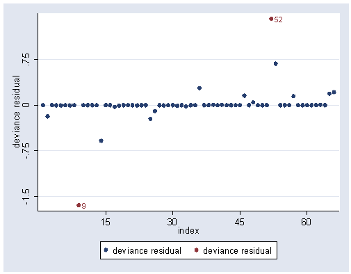
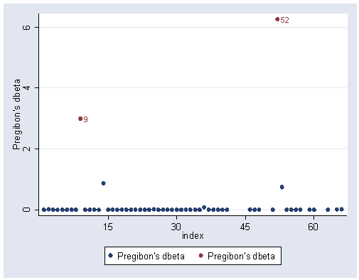
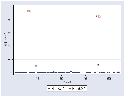
Note: Observations 9 and 52 appear to be problematic; however, observation 36
does not appear problematic, differing from the figures in the book.
sort index
graph twoway (scatter dr index) (scatter dr index if abs(dr) >= 1, mlabel(index)), ///
		ylabel(-1.5(.75).75) xlabel(15(15)60)
graph twoway (scatter dbeta index) (scatter dbeta index if abs(dbeta) >= 2, mlabel(index)), ///
		xlabel(15(15)60)
graph twoway (scatter dg index) (scatter dg index if abs(dg) >= 2, mlabel(index)), ///
		xlabel(15(15)60)
Likelihood ratio test, page 327 and table 12.3, page 328.
lrtest, saving (0)

logit y x1 x2

Logit estimates                                   Number of obs   =         66
                                                  LR chi2(2)      =      82.02
                                                  Prob > chi2     =     0.0000
Log likelihood = -4.7359473                       Pseudo R2       =     0.8965

------------------------------------------------------------------------------
       y |      Coef.   Std. Err.       z     P>|z|       [95% Conf. Interval]
---------+--------------------------------------------------------------------
      x1 |   .1573639   .0749183      2.100   0.036       .0105267    .3042011
      x2 |   .1947428   .1224281      1.591   0.112      -.0452119    .4346974
   _cons |  -.5503398   .9509818     -0.579   0.563       -2.41423     1.31355
------------------------------------------------------------------------------

Note: 11 failures and 0 successes completely determined.

lrtest

Logit:  likelihood-ratio test                         chi2(1)     =       3.66
                                                      Prob > chi2 =     0.0558
Likelihood ratio test, page 328 and table 12.4, page 328.
lrtest, saving(1)

logit y x1

Logit estimates                                   Number of obs   =         66
                                                  LR chi2(1)      =      75.69
                                                  Prob > chi2     =     0.0000
Log likelihood = -7.9015445                       Pseudo R2       =     0.8273

------------------------------------------------------------------------------
       y |      Coef.   Std. Err.       z     P>|z|       [95% Conf. Interval]
---------+--------------------------------------------------------------------
      x1 |   .1767191   .0571025      3.095   0.002       .0648004    .2886379
   _cons |  -1.166587   .8163989     -1.429   0.153        -2.7667    .4335252
------------------------------------------------------------------------------

Note: 9 failures and 0 successes completely determined.

lrtest, using(1)

Logit:  likelihood-ratio test                         chi2(1)     =       6.33
                                                      Prob > chi2 =     0.0119
Table 12.5, page 331.
regress y x1 x2 x3

  Source |       SS       df       MS                  Number of obs =      66
---------+------------------------------               F(  3,    62) =   27.38
   Model |  9.40333712     3  3.13444571               Prob > F      =  0.0000
Residual |  7.09666288    62  .114462305               R-squared     =  0.5699
---------+------------------------------               Adj R-squared =  0.5491
   Total |       16.50    65  .253846154               Root MSE      =  .33832

------------------------------------------------------------------------------
       y |      Coef.   Std. Err.       t     P>|t|       [95% Conf. Interval]
---------+--------------------------------------------------------------------
      x1 |   .0031216   .0008294      3.764   0.000       .0014637    .0047795
      x2 |   .0042457   .0014367      2.955   0.004       .0013737    .0071177
      x3 |   .1485037   .0453154      3.277   0.002       .0579195    .2390878
   _cons |   .3218658   .0874576      3.680   0.000       .1470407     .496691
------------------------------------------------------------------------------
Table 12.6, page 332.
Note: the command generate a = p >= .5 creates a new variable a which
has the value 1 if p is greater or equal to .5 and 0 otherwise.
predict p
generate a = p >= .5
list y p a

            y          p          a
  1.        0  -.0017021          0
  2.        0   .4806612          0
  3.        0   -.122117          0
  4.        0   .3064435          0
  5.        0   .2288255          0
  6.        0   .1446737          0
  7.        0   .3331264          0
  8.        0   -.320569          0
  9.        0    .517042          1
 10.        0   .1161951          0
 11.        0   .2255089          0
 12.        0  -.0724799          0
 13.        0  -.8029544          0
 14.        0    .545396          1
 15.        0   .0301355          0
 16.        0  -.4522537          0
 17.        0   .6364052          1
 18.        0   .4545762          0
 19.        0    .437882          0
 20.        0   .1398092          0
 21.        0   .2249177          0
 22.        0   .3714215          0
 23.        0   .1800966          0
 24.        0   .0519476          0
 25.        0   .5541553          1
 26.        0   .5563999          1
 27.        0    .394581          0
 28.        0   .3399023          0
 29.        0   .3882431          0
 30.        0    .262901          0
 31.        0   .3894134          0
 32.        0    .117767          0
 33.        0   .4403123          0
 34.        1   .7187779          1
 35.        1   .8186681          1
 36.        1   .7295072          1
 37.        1   .8015884          1
 38.        1   .6547927          1
 39.        1   .7962746          1
 40.        1   .7478317          1
 41.        1   .7593519          1
 42.        1   .8322027          1
 43.        1   1.099869          1
 44.        1   1.420885          1
 45.        1   .8599006          1
 46.        1    .657912          1
 47.        1   .8058342          1
 48.        1   .5835429          1
 49.        1   .9690604          1
 50.        1   1.029698          1
 51.        1   .7686977          1
 52.        1   .4763457          0
 53.        1   .5957797          1
 54.        1   .7405336          1
 55.        1   .8092653          1
 56.        1   .8389035          1
 57.        1   .6227317          1
 58.        1   .8070596          1
 59.        1   .7396857          1
 60.        1    .843024          1
 61.        1   .8565065          1
 62.        1   .7999232          1
 63.        1   .6828997          1
 64.        1   .8343272          1
 65.        1   .6078632          1
 66.        1   .5940937          1