
Table 2.3, page 25.
use https://stats.idre.ucla.edu/stat/stata/examples/chp/p025a, clear
list

             y          x
  1.         1         -7
  2.        14         -6
  3.        25         -5
  4.        34         -4
  5.        41         -3
  6.        46         -2
  7.        49         -1
  8.        50          0
  9.        49          1
 10.        46          2
 11.        41          3
 12.        34          4
 13.        25          5
 14.        14          6
 15.         1          7
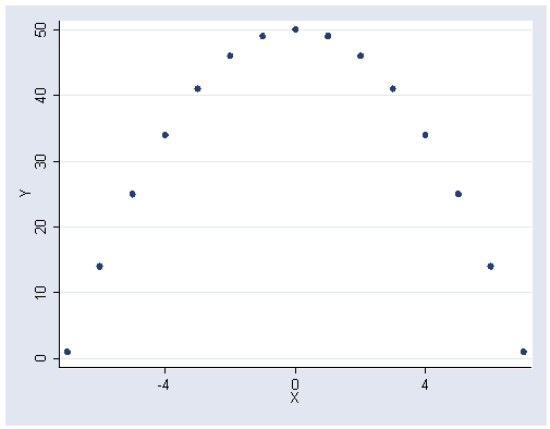
Figure 2.2, page 25.
graph twoway scatter y x, xlabel(-4 0 4)
Part of table 2.4, page 25.
use https://stats.idre.ucla.edu/stat/stata/examples/chp/p025b, clear
list y1 x1

            y1         x1
  1.      8.04         10
  2.      6.95          8
  3.      7.58         13
  4.      8.81          9
  5.      8.33         11
  6.      9.96         14
  7.      7.24          6
  8.      4.26          4
  9.     10.84         12
 10.      4.82          7
 11.      5.68          5
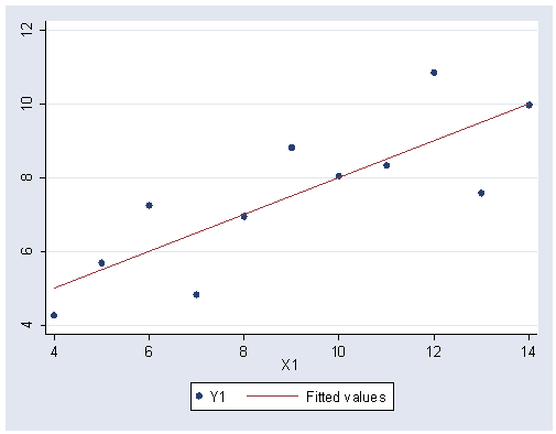
Figure 2.3(a), page 26.
graph twoway (scatter y1 x1) (lfit y1 x1)
Part of table 2.4, page 25.
list y2 x2

            y2         x2
  1.      9.14         10
  2.      8.14          8
  3.      8.74         13
  4.      8.77          9
  5.      9.26         11
  6.       8.1         14
  7.      6.13          6
  8.       3.1          4
  9.      9.13         12
 10.      7.26          7
 11.      4.74          5
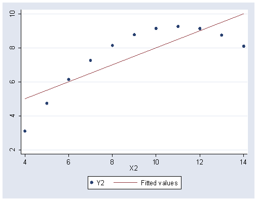
Figure 2.3(b), page 26.
graph twoway (scatter y2 x2) (lfit y2 x2)
Part of table 2.4, page 25.
list y3 x3

            y3         x3
  1.      7.46         10
  2.      6.77          8
  3.     12.74         13
  4.      7.11          9
  5.      7.81         11
  6.      8.84         14
  7.      6.08          6
  8.      5.39          4
  9.      8.15         12
 10.      6.42          7
 11.      5.73          5
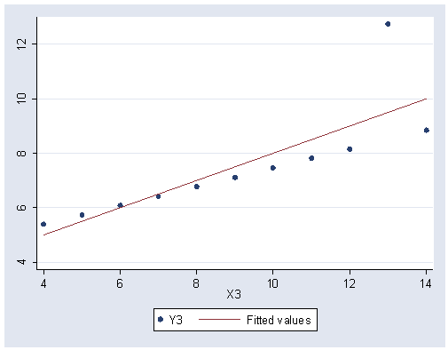
Figure 2.3(c), page 26.
graph twoway (scatter y3 x3) (lfit y3 x3)
Part of table 2.4, page 25.
list y4 x4

            y4         x4
  1.      6.58          8
  2.      5.76          8
  3.      7.71          8
  4.      8.84          8
  5.      8.47          8
  6.      7.04          8
  7.      5.25          8
  8.      12.5         19
  9.      5.56          8
 10.      7.91          8
 11.      6.89          8
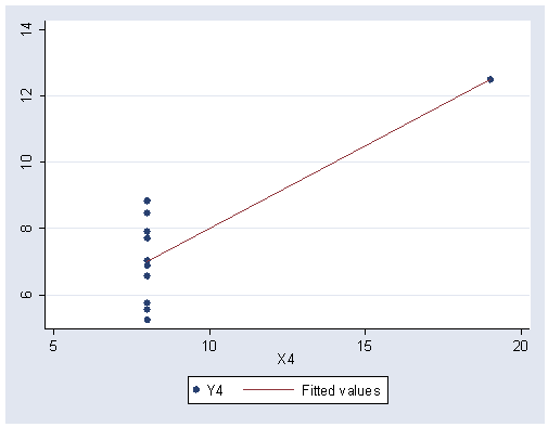
Figure 2.3(d), page 26.
graph twoway (scatter y4 x4) (lfit y4 x4)
Part of table 2.6, page 28.
use https://stats.idre.ucla.edu/stat/stata/examples/chp/p027, clear
list

       minutes      units
  1.        23          1
  2.        29          2
  3.        49          3
  4.        64          4
  5.        74          4
  6.        87          5
  7.        96          6
  8.        97          6
  9.       109          7
 10.       119          8
 11.       149          9
 12.       145          9
 13.       154         10
 14.       166         10
Commands to create remainder of table 2.6, page 28.
egen ymean = mean(minutes)        /* egen is extended generate to create a new variable */
egen xmean = mean(units)
generate ydev = minutes - ymean   /* generate creates new variables */
generate xdev = units - xmean
drop ymean xmean                  /* drop ymean and xmean, they are no longer needed */
generate ydev2 = ydev^2
generate xdev2 = xdev^2
generate yxdev = ydev*xdev
List remainder of table 2.6, page 28.
list ydev-yxdev

          ydev       xdev      ydev2      xdev2      yxdev       yhat
  1. -74.21429         -5    5507.76         25   371.0714   19.67043
  2. -68.21429         -4   4653.189         16   272.8571    35.1792
  3. -48.21429         -3   2324.617          9   144.6429   50.68797
  4. -33.21429         -2   1103.189          4   66.42857   66.19674
  5. -23.21429         -2   538.9031          4   46.42857   66.19674
  6. -10.21429         -1   104.3317          1   10.21429   81.70551
  7. -1.214287          0   1.474492          0          0   97.21429
  8. -.2142868          0   .0459188          0          0   97.21429
  9.  11.78571          1    138.903          1   11.78571   112.7231
 10.  21.78571          2   474.6173          4   43.57143   128.2318
 11.  51.78571          3    2681.76          9   155.3571   143.7406
 12.  47.78571          3   2283.474          9   143.3571   143.7406
 13.  56.78571          4   3224.617         16   227.1429   159.2494
 14.  68.78571          4   4731.474         16   275.1429   159.2494
Figure 2.4, page 28.
graph twoway scatter minutes units, ylabel(40(40)160)
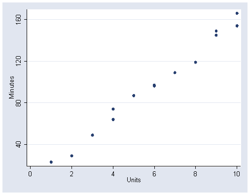
Table 2.9, page 36.
regress minutes units

  Source |       SS       df       MS                  Number of obs =      14
---------+------------------------------               F(  1,    12) =  943.20
   Model |  27419.5088     1  27419.5088               Prob > F      =  0.0000
Residual |  348.848371    12  29.0706976               R-squared     =  0.9874
---------+------------------------------               Adj R-squared =  0.9864
   Total |  27768.3571    13  2136.02747               Root MSE      =  5.3917

------------------------------------------------------------------------------
 minutes |      Coef.   Std. Err.       t     P>|t|       [95% Conf. Interval]
---------+--------------------------------------------------------------------
   units |   15.50877   .5049813     30.712   0.000       14.40851    16.60903
   _cons |   4.161654     3.3551      1.240   0.239      -3.148482    11.47179
------------------------------------------------------------------------------
Commands to produce table 2.7, page 32.
predict yhat        /* default for predict produces predicted (fitted) scores */
predict e, resid   /* resid option produces raw residuals */
Table 2.7, page 32.
list units yhat e

         units       yhat          e
  1.         1   19.67043   3.329574
  2.         2    35.1792  -6.179198
  3.         3   50.68797   -1.68797
  4.         4   66.19674  -2.196742
  5.         4   66.19674   7.803258
  6.         5   81.70551   5.294486
  7.         6   97.21429  -1.214286
  8.         6   97.21429  -.2142857
  9.         7   112.7231  -3.723058
 10.         8   128.2318   -9.23183
 11.         9   143.7406   5.259398
 12.         9   143.7406   1.259398
 13.        10   159.2494  -5.249373
 14.        10   159.2494   6.750627
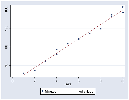
Figure 2.5, page 32.
graph twoway (scatter minutes units) (lfit minutes units), ylabel(40(40)160)
The confidence interval on page 38 included in table 2.9 above.
Standard error for a predicted score, page 39.
predict seyhat, stdf
list seyhat

        seyhat
  1.  6.125547
  2.  5.935257
  3.  5.782926
  4.  5.671614
  5.  5.671614
  6.  5.603765
  7.  5.580966
  8.  5.580966
  9.  5.603765
 10.  5.671614
 11.  5.782926
 12.  5.782926
 13.  5.935257
 14.  5.935257
Standard error for mean prediction, page 39.
predict semu, stdp
list semu

       minutes      units       semu
  1.        23          1   2.907169
  2.        29          2   2.481245
  3.        49          3   2.090821
  4.        64          4   1.759688
  5.        74          4   1.759688
  6.        87          5    1.52692
  7.        96          6   1.440999
  8.        97          6   1.440999
  9.       109          7    1.52692
 10.       119          8   1.759688
 11.       149          9   2.090821
 12.       145          9   2.090821
 13.       154         10   2.481245
 14.       166         10   2.481245
Correlations, page 43.
correlat minutes units
(obs=14)

         |  minutes    units
---------+------------------
 minutes |   1.0000
   units |   0.9937   1.0000

correlate minutes yhat
(obs=14)

         |  minutes     yhat
---------+------------------
 minutes |   1.0000
    yhat |   0.9937   1.0000
Correlation squared, page 43.
Note: The display command demonstrates Stata’s ability to function as a calculator.
display .9937^2
.98743969
R-squared from regression sums of squares, page 43.
Note: This display uses values e(rss) and e(mss) saved by the regression command.
It will work only after the regression has been estimated.
display 1 - (e(rss)/(e(rss)+e(mss)))
.9874372
Save the modified data file p027.
save p027, replace