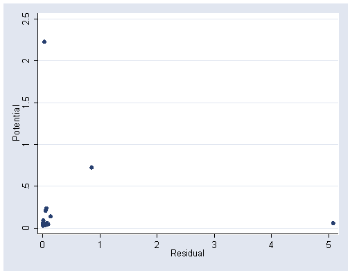
Figure 4.1, page 91.
Duplicates figure 2.3 from Chapter 2.
use https://stats.idre.ucla.edu/stat/stata/examples/chp/p095, clear
Table 4.1, page 95.
list

             y         x1         x2
  1.     12.37       2.23       9.66
  2.     12.66       2.57       8.94
  3.        12       3.87        4.4
  4.     11.93        3.1       6.64
..
  [remainder of output omitted]
Figure 4.2, page 94. Provide the graph command but we are not displaying the output.
corr y x1 x2
(obs=15)

         |        y       x1       x2
---------+---------------------------
       y |   1.0000
      x1 |   0.0025   1.0000
      x2 |   0.4341  -0.8998   1.0000

graph matrix y x1 x2, half
Coefficients for page 95.
regress y x1

  Source |       SS       df       MS                  Number of obs =      15
---------+------------------------------               F(  1,    13) =    0.00
   Model |  .000056215     1  .000056215               Prob > F      =  0.9930
Residual |   9.0085422    13  .692964784               R-squared     =  0.0000
---------+------------------------------               Adj R-squared = -0.0769
   Total |  9.00859841    14  .643471315               Root MSE      =  .83245

------------------------------------------------------------------------------
       y |      Coef.   Std. Err.       t     P>|t|       [95% Conf. Interval]
---------+--------------------------------------------------------------------
      x1 |   .0037476   .4160825      0.009   0.993      -.8951439    .9026391
   _cons |   11.98875   1.266891      9.463   0.000       9.251804    14.72571
------------------------------------------------------------------------------

regress y x2

  Source |       SS       df       MS                  Number of obs =      15
---------+------------------------------               F(  1,    13) =    3.02
   Model |   1.6973605     1   1.6973605               Prob > F      =  0.1060
Residual |  7.31123791    13  .562402916               R-squared     =  0.1884
---------+------------------------------               Adj R-squared =  0.1260
   Total |  9.00859841    14  .643471315               Root MSE      =  .74994

------------------------------------------------------------------------------
       y |      Coef.   Std. Err.       t     P>|t|       [95% Conf. Interval]
---------+--------------------------------------------------------------------
      x2 |   .1954562   .1125087      1.737   0.106      -.0476041    .4385165
   _cons |   10.63194   .8109425     13.111   0.000       8.880002    12.38387
------------------------------------------------------------------------------

regress y x1 x2

  Source |       SS       df       MS                  Number of obs =      15
---------+------------------------------               F(  2,    12) =39222.21
   Model |  9.00722053     2  4.50361027               Prob > F      =  0.0000
Residual |  .001377876    12  .000114823               R-squared     =  0.9998
---------+------------------------------               Adj R-squared =  0.9998
   Total |  9.00859841    14  .643471315               Root MSE      =  .01072

------------------------------------------------------------------------------
       y |      Coef.   Std. Err.       t     P>|t|       [95% Conf. Interval]
---------+--------------------------------------------------------------------
      x1 |   3.097008   .0122745    252.313   0.000       3.070264    3.123752
      x2 |   1.031859   .0036842    280.078   0.000       1.023832    1.039886
   _cons |  -4.515414   .0611419    -73.851   0.000      -4.648631   -4.382198
------------------------------------------------------------------------------
t-test for table 4.2, page 99.
use https://stats.idre.ucla.edu/stat/stata/examples/chp/p010
regress nitrogen agr forest rsdntial comindl

  Source |       SS       df       MS                  Number of obs =      20
---------+------------------------------               F(  4,    15) =    9.15
   Model |  2.56984613     4  .642461533               Prob > F      =  0.0006
Residual |   1.0527287    15  .070181913               R-squared     =  0.7094
---------+------------------------------               Adj R-squared =  0.6319
   Total |  3.62257483    19  .190661833               Root MSE      =  .26492

------------------------------------------------------------------------------
nitrogen |      Coef.   Std. Err.       t     P>|t|       [95% Conf. Interval]
---------+--------------------------------------------------------------------
     agr |   .0058091    .015034      0.386   0.705       -.026235    .0378533
  forest |  -.0129679   .0139315     -0.931   0.367      -.0426621    .0167264
rsdntial |  -.0072268     .03383     -0.214   0.834      -.0793338    .0648803
 comindl |   .3050278   .1638167      1.862   0.082      -.0441392    .6541947
   _cons |   1.722214   1.234082      1.396   0.183       -.908169    4.352596
------------------------------------------------------------------------------

regress nitrogen agr forest rsdntial comindl if river ~= "Neversink"

  Source |       SS       df       MS                  Number of obs =      19
---------+------------------------------               F(  4,    14) =   20.76
   Model |  3.07765167     4  .769412918               Prob > F      =  0.0000
Residual |  .518811319    14  .037057951               R-squared     =  0.8557
---------+------------------------------               Adj R-squared =  0.8145
   Total |  3.59646299    18  .199803499               Root MSE      =   .1925

------------------------------------------------------------------------------
nitrogen |      Coef.   Std. Err.       t     P>|t|       [95% Conf. Interval]
---------+--------------------------------------------------------------------
     agr |   .0101367   .0109838      0.923   0.372      -.0134213    .0336947
  forest |  -.0075892   .0102221     -0.742   0.470      -.0295134    .0143349
rsdntial |  -.1237929    .039337     -3.147   0.007      -.2081624   -.0394234
 comindl |   1.528956   .3437191      4.448   0.001       .7917521     2.26616
   _cons |   1.099471   .9116357      1.206   0.248      -.8557928    3.054735
------------------------------------------------------------------------------

regress nitrogen agr forest rsdntial comindl if river ~= "Hackensack"

  Source |       SS       df       MS                  Number of obs =      19
---------+------------------------------               F(  4,    14) =   22.24
   Model |  2.49968384     4  .624920959               Prob > F      =  0.0000
Residual |  .393358087    14  .028097006               R-squared     =  0.8640
---------+------------------------------               Adj R-squared =  0.8252
   Total |  2.89304192    18  .160724551               Root MSE      =  .16762

------------------------------------------------------------------------------
nitrogen |      Coef.   Std. Err.       t     P>|t|       [95% Conf. Interval]
---------+--------------------------------------------------------------------
     agr |   .0023522   .0095391      0.247   0.809      -.0181072    .0228117
  forest |  -.0127603   .0088149     -1.448   0.170      -.0316665    .0061458
rsdntial |    .181161     .04439      4.081   0.001       .0859538    .2763682
 comindl |   .0756176   .1139572      0.664   0.518      -.1687963    .3200315
   _cons |   1.626014   .7810911      2.082   0.056      -.0492596    3.301288
------------------------------------------------------------------------------
Figure 4.5, page 102.
gen n = _n. graph twoway (scatter nitrogen comindl, mlabel(n)) (lfit nitrogen comindl)
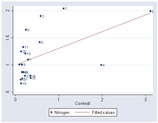
Table 4.3, page 103.
predict r, rstandard

list r p

             r       phat
  1.   .032278   1.088083
  2. -.0450231   1.026516
  3.  1.952922   1.177355
  4. -1.847232   1.608324
  5.   .155291   1.956178
  6.  .6723057   1.171199
  7.  1.923264   1.340508
  8.  1.565621   1.072691
  9. -.0951495   1.044986
 10.  .3808243   1.069613
 11.  .7492378   1.054221
 12. -.8103347   1.048065
 13. -.8324621   1.035751
 14. -.8293861   1.106553
 15. -.9376069   1.106553
 16.  -.475896   1.044986
 17. -.7232284   1.066535
 18. -.5004942   1.054221
 19. -1.031034    1.03883
 20.  .5747275    1.03883
Figure 4.6(a), page 103.
Note: The yline option draws a horizontal line at zero.
graph twoway (scatter r n), yline(0) xlabel(1(2)19)
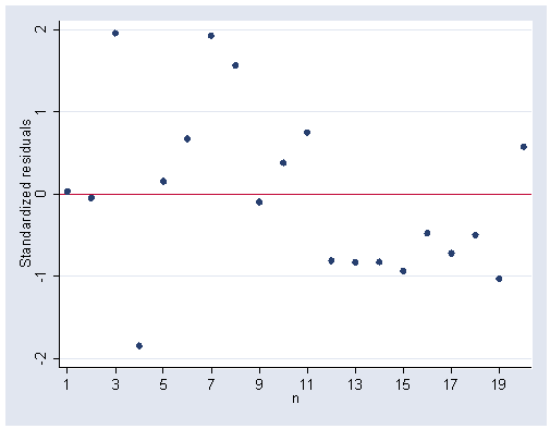
Figure 4.6(b), page 103.
graph twoway (scatter hat n), xlabel(1(2)19)
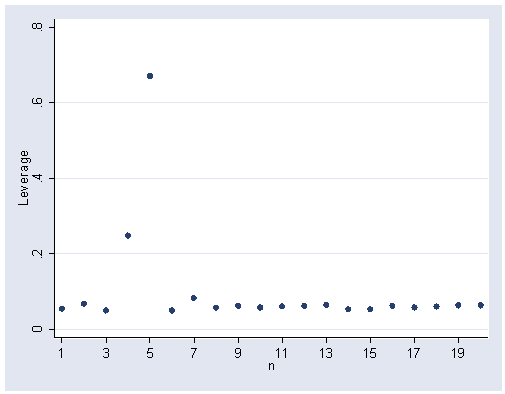
Table 4.4, page 106.
Note 1: The hinflu6 command, which generates the Hadi influence measure, is an
updated version of a command published in Stata Technical Bulletin 6. The
hinflu can be downloaded from UCLA ATS from within Stata (see
How can I use the search command to search for programs and get additional
help? for more information about using search).Note 2: The sort command was used to return the data back to their original order.
predict c, cooks
predict dfits, dfits
hinflu6 h
sort n
list c dfits h

             c      dfits          h
  1.  .0000301   .0075454   .0579712
  2.  .0000724   -.011698   .0716953
  3.  .1011772   .4924355   .5835671
  4.  .5622548  -1.144754   .7717384
  5.  .0245928   .2156743   2.042283
  6.  .0119404   .1521018   .1042828
  7.  .1665338    .629226   .5965196
  8.   .074084   .4024879   .3729268
  9.  .0003009  -.0238455   .0674733
 10.  .0044255   .0917998   .0772676
 11.  .0180378   .1875317   .1285208
 12.  .0215743  -.2056559   .1412572
 13.  .0238624   -.216514   .1487441
 14.  .0190677  -.1935145   .1347416
 15.  .0243684  -.2199832   .1578567
 16.  .0075266   -.119992   .0919314
 17.  .0161191  -.1770831   .1213872
 18.   .008049  -.1241701   .0924663
 19.  .0361671  -.2694501   .1930732
 20.  .0112381    .147052   .1053881
Figure 4.7(a), page 107.
graph twoway scatter c n, xlabel(4(4)20) ylabel(.1(.1).5)
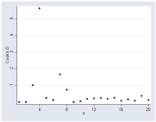
Figure 4.7(b), page 107.
graph twoway scatter dfits n, xlabel(4(4)20) ylabel(-1.2(.4).4)
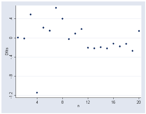
Figure 4.7(c), page 107.
graph twoway scatter h n, xlabel(4(4)20) ylabel(0(.5)2)
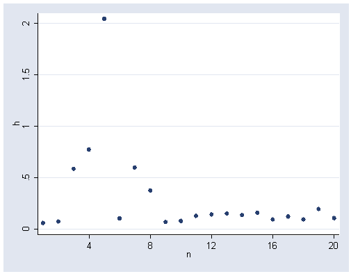
Figure 4.8, page 108.
Note: The hadiplot command can be from within Stata as shown below. You can download this program from within Stata by
typing search hadiplot (see
How can I use the search command to search for programs and get additional
help? for more information about using search).
hadiplot
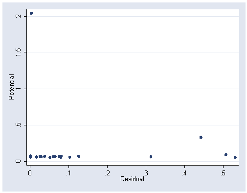
Equation 4.25, page 111.
use https://stats.idre.ucla.edu/stat/stata/examples/chp/p112, clear
regress time distance climb

  Source |       SS       df       MS                  Number of obs =      35
---------+------------------------------               F(  2,    32) =  181.66
   Model |   281686567     2   140843283               Prob > F      =  0.0000
Residual |  24810081.9    32  775315.059               R-squared     =  0.9191
---------+------------------------------               Adj R-squared =  0.9140
   Total |   306496649    34  9014607.31               Root MSE      =  880.52

------------------------------------------------------------------------------
    time |      Coef.   Std. Err.       t     P>|t|       [95% Conf. Interval]
---------+--------------------------------------------------------------------
distance |   373.0727   36.06841     10.343   0.000       299.6037    446.5416
   climb |    .662888   .1230519      5.387   0.000       .4122395    .9135365
   _cons |  -539.4829   258.1607     -2.090   0.045      -1065.339   -13.62671
------------------------------------------------------------------------------
Figure 4.11, page 114.
avplots
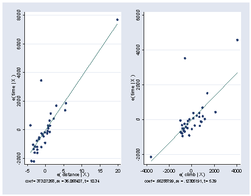
Figure 4.12(a), page 114.
Note: The graph in the book is incorrect,
see errata .
cprplot distance
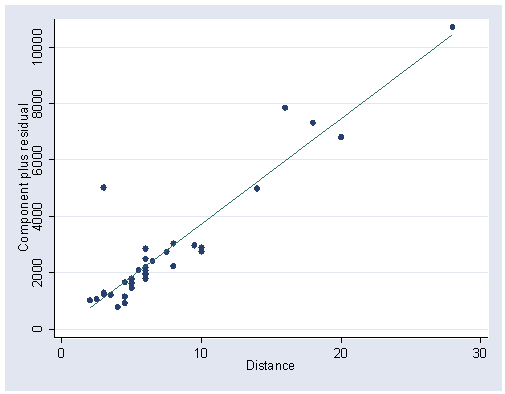
Figure 4.12(b), page 114.
Note: The graph in the book is incorrect,
see errata .
cprplot climb
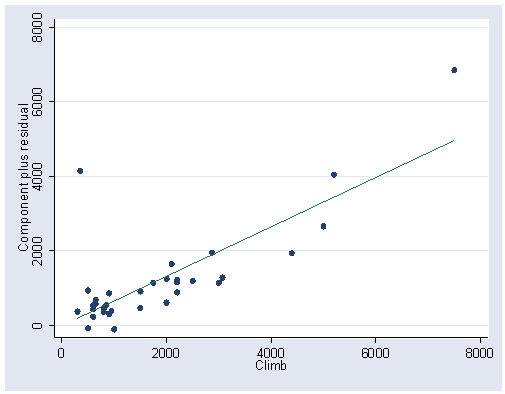
Figure 4.13, page 114.
hadiplot