Note: The generate command is used to add an id number to the observations.
use https://stats.idre.ucla.edu/stat/stata/examples/chp/p124

generate id = _n
Table 5.1, page 124.
list

            s         x         e         m
  1.    13876         1         1         1
  2.    11608         1         3         0
  3.    18701         1         3         1
  4.    11283         1         2         0
  5.    11767         1         3         0
  6.    20872         2         2         1
  7.    11772         2         2         0
  8.    10535         2         1         0
  9.    12195         2         3         0
 10.    12313         3         2         0
..
  [remainder of output omitted]
Create dummy coding for variable e.
Note 1: tabulate with the generate option creates dummy coded variables.
Note 2: The tab1 command produces one-way frequency tables for a series of variables.
tabulate e, generate(e)

          E |      Freq.     Percent        Cum.
------------+-----------------------------------
          1 |         14       30.43       30.43
          2 |         19       41.30       71.74
          3 |         13       28.26      100.00
------------+-----------------------------------
      Total |         46      100.00

tab1 e1 e2 e3

-> tabulation of e1

        e== |
     1.0000 |      Freq.     Percent        Cum.
------------+-----------------------------------
          0 |         32       69.57       69.57
          1 |         14       30.43      100.00
------------+-----------------------------------
      Total |         46      100.00

-> tabulation of e2

        e== |
     2.0000 |      Freq.     Percent        Cum.
------------+-----------------------------------
          0 |         27       58.70       58.70
          1 |         19       41.30      100.00
------------+-----------------------------------
      Total |         46      100.00

-> tabulation of e3

        e== |
     3.0000 |      Freq.     Percent        Cum.
------------+-----------------------------------
          0 |         33       71.74       71.74
          1 |         13       28.26      100.00
------------+-----------------------------------
      Total |         46      100.00
Table 5.3, page 126.
regress s x e1 e2 m

  Source |       SS       df       MS                  Number of obs =      46
---------+------------------------------               F(  4,    41) =  226.84
   Model |   957816858     4   239454214               Prob > F      =  0.0000
Residual |  43280719.5    41  1055627.30               R-squared     =  0.9568
---------+------------------------------               Adj R-squared =  0.9525
   Total |  1.0011e+09    45  22246612.8               Root MSE      =  1027.4

------------------------------------------------------------------------------
       s |      Coef.   Std. Err.       t     P>|t|       [95% Conf. Interval]
---------+--------------------------------------------------------------------
       x |    546.184   30.51919     17.896   0.000       484.5493    607.8188
      e1 |   -2996.21   411.7527     -7.277   0.000      -3827.762   -2164.659
      e2 |   147.8249   387.6593      0.381   0.705      -635.0689    930.7188
       m |   6883.531    313.919     21.928   0.000       6249.559    7517.503
   _cons |   11031.81   383.2171     28.787   0.000       10257.89    11805.73
------------------------------------------------------------------------------
Figure 5.1, page 127. The rvpplot2 can be downloaded within Stata by typing search
rvpplot2 (see How can I use the search
command to search for programs and get additional help? for more
information about using search).
rvpplot2 x, rstudent xlabel(4(4)20) ylabel(-2(1)1)
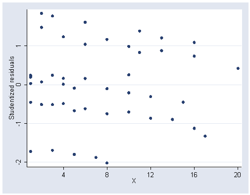
Figure 5.2, page 128.
Note 1: The egen command was used with the group function to produce the six
categories of education and management.Note 2: The xlabel(1(1)6) option produces labels on the x-axis from 1 to 6 by ones.
egen c = group(e m)
predict sr, rstandard
graph twoway scatter sr c, ylabel(-2(1)1) xlabel(1(1)6)
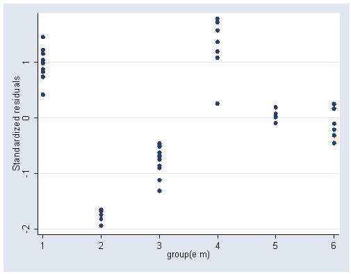
Table 5.4, page 129.
generate e1m = e1*m
generate e2m = e2*m
regress s x e1 e2 m e1m e2m

  Source |       SS       df       MS                  Number of obs =      46
---------+------------------------------               F(  6,    39) = 5516.60
   Model |   999919409     6   166653235               Prob > F      =  0.0000
Residual |  1178167.86    39  30209.4324               R-squared     =  0.9988
---------+------------------------------               Adj R-squared =  0.9986
   Total |  1.0011e+09    45  22246612.8               Root MSE      =  173.81

------------------------------------------------------------------------------
       s |      Coef.   Std. Err.       t     P>|t|       [95% Conf. Interval]
---------+--------------------------------------------------------------------
       x |    496.987   5.566415     89.283   0.000       485.7279    508.2461
      e1 |  -1730.748   105.3339    -16.431   0.000      -1943.806    -1517.69
      e2 |  -349.0777    97.5679     -3.578   0.001      -546.4274    -151.728
       m |   7047.412   102.5892     68.695   0.000       6839.906    7254.918
     e1m |  -3066.035   149.3304    -20.532   0.000      -3368.084   -2763.986
     e2m |   1836.488   131.1674     14.001   0.000       1571.177    2101.799
   _cons |   11203.43   79.06545    141.698   0.000       11043.51    11363.36
------------------------------------------------------------------------------
Figure 5.3, page 129.
rvpplot2 x, rstandard xlabel(4(4)20) ylabel(-6(1.5)1.5)
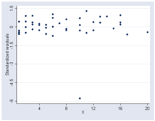
Table 5.5, page 129.
drop if id==33
(1 observation deleted)

regress s x e1 e2 m e1m e2m

  Source |       SS       df       MS                  Number of obs =      45
---------+------------------------------               F(  6,    38) =35427.96
   Model |   957607113     6   159601186               Prob > F      =  0.0000
Residual |   171188.12    38  4504.95052               R-squared     =  0.9998
---------+------------------------------               Adj R-squared =  0.9998
   Total |   957778301    44  21767688.7               Root MSE      =  67.119

------------------------------------------------------------------------------
       s |      Coef.   Std. Err.       t     P>|t|       [95% Conf. Interval]
---------+--------------------------------------------------------------------
       x |   498.4178   2.151688    231.640   0.000       494.0619    502.7736
      e1 |  -1741.336    40.6825    -42.803   0.000      -1823.693   -1658.979
      e2 |  -357.0423   37.68114     -9.475   0.000      -433.3237   -280.7608
       m |    7040.58   39.61907    177.707   0.000       6960.376    7120.785
     e1m |  -3051.763    57.6742    -52.914   0.000      -3168.519   -2935.008
     e2m |   1997.531   51.78498     38.574   0.000       1892.697    2102.364
   _cons |   11199.71   30.53338    366.802   0.000        11137.9    11261.53
------------------------------------------------------------------------------
Figure 5.4, page 130.
rvpplot2 x, rstandard xlabel(4(4)20) ylabel(-2(1)2)
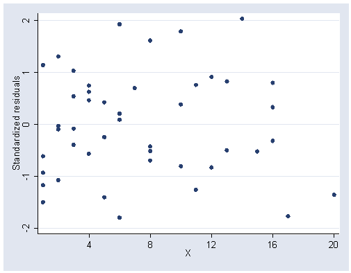
Figure 5.5, page 130.
drop sr
predict sr, rstandard
graph twoway scatter sr c, ylabel(-2(1)1) xlabel(1(1)6)
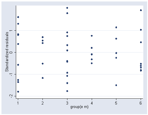
Table 5.6, page 131.
Note: There are small differences between table 5.6 in the book and the one
generated by Stata due to rounding.
adjust x=0, by(m e) se ci format(%5.0f)

-------------------------------------------------------------------------------
Dependent variable: s     Command: regress
Variables left as is: e1, e2, e1m, e2m
Covariate set to value: x = 0
-------------------------------------------------------------------------------

----------+--------------------------------------------
          |                      E
        M |             1              2              3
----------+--------------------------------------------
        0 |          9458          10843          11200
          |          (31)           (26)           (31)
          |   [9396,9521]  [10790,10896]  [11138,11262]
          |
        1 |         13447          19881          18240
          |          (32)           (33)           (29)
          | [13383,13511]  [19814,19947]  [18183,18298]
----------+--------------------------------------------
Use the data file p134 and create interaction variable.
use https://stats.idre.ucla.edu/stat/stata/examples/chp/p134, clear

generate rbyt = race*test
Table 5.8, page 135.
regress jperf test

  Source |       SS       df       MS                  Number of obs =      20
---------+------------------------------               F(  1,    18) =   19.25
   Model |  48.7229625     1  48.7229625               Prob > F      =  0.0004
Residual |  45.5682959    18    2.531572               R-squared     =  0.5167
---------+------------------------------               Adj R-squared =  0.4899
   Total |  94.2912585    19  4.96269781               Root MSE      =  1.5911

------------------------------------------------------------------------------
   jperf |      Coef.   Std. Err.       t     P>|t|       [95% Conf. Interval]
---------+--------------------------------------------------------------------
    test |   2.360535   .5380699      4.387   0.000       1.230092    3.490978
   _cons |   1.034973   .8680312      1.192   0.249      -.7886928    2.858639
------------------------------------------------------------------------------
Figure 5.7, page 135.
rvpplot2 test, rstandard ylabel(-2(1)1) xlabel(.75 1.5 2.25)
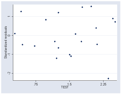
Figure 5.9, page 137.
predict sr, rstandard
graph twoway scatter sr race, ylabel(-2(1)1) xlabel(0 1)
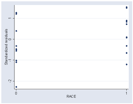
Table 5.9, page 135.
regress jperf test race rbyt

  Source |       SS       df       MS                  Number of obs =      20
---------+------------------------------               F(  3,    16) =   10.55
   Model |  62.6357847     3  20.8785949               Prob > F      =  0.0005
Residual |  31.6554738    16  1.97846711               R-squared     =  0.6643
---------+------------------------------               Adj R-squared =  0.6013
   Total |  94.2912585    19  4.96269781               Root MSE      =  1.4066

------------------------------------------------------------------------------
   jperf |      Coef.   Std. Err.       t     P>|t|       [95% Conf. Interval]
---------+--------------------------------------------------------------------
    test |   1.313402   .6703711      1.959   0.068      -.1077208    2.734525
    race |  -1.913167   1.540325     -1.242   0.232      -5.178509    1.352176
    rbyt |   1.997546    .954443      2.093   0.053      -.0257831    4.020875
   _cons |   2.010282   1.050112      1.914   0.074      -.2158562    4.236421
------------------------------------------------------------------------------
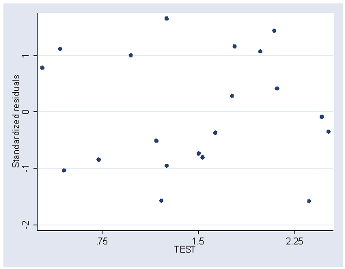
Figure 5.8, page 135.
rvpplot2 test, rstandard ylabel(-2(1)1) xlabel(.75 1.5 2.25)
Part of Table 5.10, page 136.
regress jperf test if race==1

  Source |       SS       df       MS                  Number of obs =      10
---------+------------------------------               F(  1,     8) =   28.14
   Model |  46.9895716     1  46.9895716               Prob > F      =  0.0007
Residual |  13.3568411     8  1.66960513               R-squared     =  0.7787
---------+------------------------------               Adj R-squared =  0.7510
   Total |  60.3464126     9  6.70515696               Root MSE      =  1.2921

------------------------------------------------------------------------------
   jperf |      Coef.   Std. Err.       t     P>|t|       [95% Conf. Interval]
---------+--------------------------------------------------------------------
    test |   3.310948   .6241062      5.305   0.001       1.871757     4.75014
   _cons |   .0971152   1.035193      0.094   0.928      -2.290043    2.484274
------------------------------------------------------------------------------

------------------------------------------------------------------------------
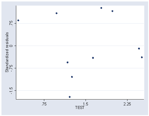
Figure 5.10, page 137.
rvpplot2 test, rstandard ylabel(-1.5(.75).75) xlabel(.75 1.5 2.25)
Remainder of Table 5.10, page 136.
regress jperf test if race==0

  Source |       SS       df       MS                  Number of obs =      10
---------+------------------------------               F(  1,     8) =    3.32
   Model |   7.5944073     1   7.5944073               Prob > F      =  0.1059
Residual |  18.2986327     8  2.28732909               R-squared     =  0.2933
---------+------------------------------               Adj R-squared =  0.2050
   Total |    25.89304     9  2.87700445               Root MSE      =  1.5124

------------------------------------------------------------------------------
   jperf |      Coef.   Std. Err.       t     P>|t|       [95% Conf. Interval]
---------+--------------------------------------------------------------------
    test |   1.313402   .7208006      1.822   0.106      -.3487669    2.975572
   _cons |   2.010282   1.129108      1.780   0.113      -.5934463    4.614011
------------------------------------------------------------------------------
Figure 5.11, page 137.
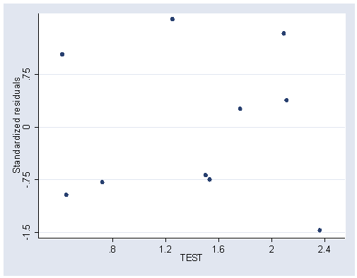
rvpplot2 test, rstandard ylabel(-1.5(.75).75) xlabel(.8(.4)2.4)