
Table 9.3-1, page 369
use https://stats.idre.ucla.edu/stat/stata/examples/kirk/crf33, clear

tabdisp order b a, cellvar(y)

----------+---------------------------------------------------------
          |                         a and b
          | ------- 1 ------    ------- 2 ------    ------- 3 ------
    order |    1     2     3       1     2     3       1     2     3
----------+---------------------------------------------------------
        1 |   24    44    38      30    35    26      21    41    42
        2 |   33    36    29      21    40    27      18    39    52
        3 |   37    25    28      39    27    36      10    50    53
        4 |   29    27    47      26    31    46      31    36    49
        5 |   42    43    48      34    22    45      20    34    64
----------+---------------------------------------------------------

table a b, cont(sum y)

----------+-----------------
          |        b
        a |    1     2     3
----------+-----------------
        1 |  165   175   190
        2 |  150   155   180
        3 |  100   200   260
----------+-----------------
Table 9.3-2, page 370
anova y a b a*b

                     Number of obs =      45     R-squared     =  0.5690
                     Root MSE      = 7.90569     Adj R-squared =  0.4732

            Source |  Partial SS    df       MS           F     Prob > F
        -----------+----------------------------------------------------
             Model |     2970.00     8      371.25       5.94     0.0001
                   |
                 a |      190.00     2       95.00       1.52     0.2324
                 b |  1543.33333     2  771.666667      12.35     0.0001
               a*b |  1236.66667     4  309.166667       4.95     0.0028
                   |
          Residual |     2250.00    36       62.50
        -----------+----------------------------------------------------
             Total |     5220.00    44  118.636364
Figure 9.3-1, page 371
Note: You can download anovaplot
from within Stata by typing search anovaplot (see
How can I use the search command to search
for programs and get additional help? for more information about using
search).
anovaplot, scatter(msymbol(i)) /* Figure 9.3-1 (a) */
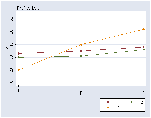
quietly anova y a b a*b
anovaplot, scatter(msymbol(i))  /* Figure 9.3-1 (b) */
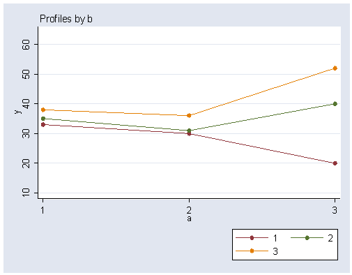
Table 9.6-2, page 380
Note: The sme command can be downloaded by typing search contrast (see
How can I use the search command to search for programs and get additional help? for more information about using
search).
sme a b

Test of a at b(1): F(2/36)  = 3.7066667
Test of a at b(2): F(2/36)  = 1.6266667
Test of a at b(3): F(2/36)  = 6.08


Critical value of F for alpha = .05 using ...
--------------------------------------------------
Dunn's procedure              = 4.0941238
Marascuilo & Levin            = 4.5974255
per family error rate         = 4.5974255
simultaneous test procedure   = 6.5295994

sme b a

Test of b at a(1): F(2/36)  = .50666667
Test of b at a(2): F(2/36)  = .82666667
Test of b at a(3): F(2/36)  = 20.906667


Critical value of F for alpha = .05 using ...
--------------------------------------------------
Dunn's procedure              = 4.0941238
Marascuilo & Levin            = 4.5974255
per family error rate         = 4.5974255
simultaneous test procedure   = 6.5295994
Omega-squared computations, page 397.
Note: The omega2 command can be downloaded by typing search contrast (see
How can I use the search command to search for programs and get additional help? for more information about using
search).
omega2 1.52 2  /* see Kirk, page 399, for formula */

 omega squared = 0.0226
 effect size   = 0.1520

omega2 12.35 2

 omega squared = 0.3353
 effect size   = 0.7102

omega2 4.95 4

 omega squared = 0.2599
 effect size   = 0.5925
Table 8-14-1, page 423
use https://stats.idre.ucla.edu/stat/stata/examples/kirk/crf33a, clear

tabdisp order b a, cellvar(y)

----------+---------------------------------------------------------
          |                         a and b
          | ------- 1 ------    ------- 2 ------    ------- 3 ------
    order |    1     2     3       1     2     3       1     2     3
----------+---------------------------------------------------------
        1 |   24    44    38      30    35    26      21    41    42
        2 |   33    36    29      21    40    27      18    39    52
        3 |   37    25    28      39    27    36      10    50    53
        4 |   29    27    47      26    31    46      31    36    49
        5 |         43    48      34    22    45      20    34    64
----------+---------------------------------------------------------

table a b, cont(freq mean y)

----------+--------------------
          |          b
        a |     1      2      3
----------+--------------------
        1 |     4      5      5
          | 30.75     35     38
          |
        2 |     5      5      5
          |    30     31     36
          |
        3 |     5      5      5
          |    20     40     52
----------+--------------------
SSA, page 424
anova y a b a*b, sequential

                     Number of obs =      44     R-squared     =  0.5844
                     Root MSE      = 7.83536     Adj R-squared =  0.4894

            Source |    Seq. SS     df       MS           F     Prob > F
        -----------+----------------------------------------------------
             Model |  3021.13636     8  377.642045       6.15     0.0001
                   |
                 a |  187.505411     2  93.7527056       1.53     0.2313
                 b |  1716.21429     2  858.107143      13.98     0.0000
               a*b |  1117.41667     4  279.354167       4.55     0.0046
                   |
          Residual |     2148.75    35  61.3928571
        -----------+----------------------------------------------------
             Total |  5169.88636    43  120.229915
SSB and SSAB, page 425
anova y b a a*b, sequential

                     Number of obs =      44     R-squared     =  0.5844
                     Root MSE      = 7.83536     Adj R-squared =  0.4894

            Source |    Seq. SS     df       MS           F     Prob > F
        -----------+----------------------------------------------------
             Model |  3021.13636     8  377.642045       6.15     0.0001
                   |
                 b |  1713.33874     2  856.669372      13.95     0.0000
                 a |  190.380952     2  95.1904762       1.55     0.2264
               a*b |  1117.41667     4  279.354167       4.55     0.0046
                   |
          Residual |     2148.75    35  61.3928571
        -----------+----------------------------------------------------
             Total |  5169.88636    43  120.229915