
use https://stats.idre.ucla.edu/stat/stata/examples/methods_matter/chapter8/dynarski, clear
svyset, clear
svyset [pw=wt88], psu(hhid)

      pweight: wt88
          VCE: linearized
  Single unit: missing
     Strata 1: <one>
         SU 1: hhid
        FPC 1: <zero>
Descriptive statistics and cross-tabulations for key variables. (Not shown in text.)
svy: mean coll
(running mean on estimation sample)

Survey: Mean estimation

Number of strata =       1      Number of obs    =        3986
Number of PSUs   =    3123      Population size  =  1302933368
                                Design df        =        3122

--------------------------------------------------------------
             |             Linearized
             |       Mean   Std. Err.     [95% Conf. Interval]
-------------+------------------------------------------------
        coll |   .4943504   .0105154      .4737326    .5149681
--------------------------------------------------------------

tabulate fatherdec yearsr

 Father deceased by |                 Year in which a senior
             age 18 |        79         80         81         82         83 |     Total
--------------------+-------------------------------------------------------+----------
Father not deceased |       892        986        867        828        222 |     3,795
    Father deceased |        41         44         52         41         13 |       191
--------------------+-------------------------------------------------------+----------
              Total |       933      1,030        919        869        235 |     3,986
(a) Direct Estimate shown in Table 8.1 on page
143. The means of coll are shown in the rows labeled _subpop_3 and
_subpop_4. This output also replicates part of the table of variable means and differences from the Dynarski article referenced in the chapter
(not shown in the text).
svy: mean coll, over(fatherdec offer)
(running mean on estimation sample)

Survey: Mean estimation

Number of strata =       1      Number of obs    =        3986
Number of PSUs   =    3123      Population size  =  1302933368
                                Design df        =        3122

         Over: fatherdec offer
    _subpop_1: Father not deceased 0
    _subpop_2: Father not deceased 1
    _subpop_3: Father deceased 0
    _subpop_4: Father deceased 1

--------------------------------------------------------------
             |             Linearized
        Over |       Mean   Std. Err.     [95% Conf. Interval]
-------------+------------------------------------------------
coll         |
   _subpop_1 |   .4756935   .0188649      .4387046    .5126825
   _subpop_2 |   .5017016   .0121735      .4778327    .5255706
   _subpop_3 |   .3522178   .0812446      .1929197     .511516
   _subpop_4 |   .5604556   .0527439      .4570394    .6638718
-------------+------------------------------------------------
(b) Linear-Probability Model (OLS) Estimate shown in Table 8.1 on page 143.
svy if fatherdec==1 : regress coll offer
(running regress on estimation sample)

Survey: Linear regression

Number of strata   =         1                  Number of obs      =       191
Number of PSUs     =       172                  Population size    =  51656801
                                                Design df          =       171
                                                F(   1,    171)    =      4.96
                                                Prob > F           =    0.0272
                                                R-squared          =    0.0358

------------------------------------------------------------------------------
             |             Linearized
        coll |      Coef.   Std. Err.      t    P>|t|     [95% Conf. Interval]
-------------+----------------------------------------------------------------
       offer |   .2082378   .0935031     2.23   0.027     .0236689    .3928067
       _cons |   .3522178   .0814687     4.32   0.000      .191404    .5130317
------------------------------------------------------------------------------
Figure 8.1 on page 155.
recode offer (0=1) (1=0), gen(post)

twoway lfit coll post [pw=wt88], by(fatherdec, note("")) ///
	ytitle("P{college}") yscale(range(.3 .6)) ///
	xtitle("Year") xlabel(0 "Pre-1981" 1 "Post-1981") xscale(range(-.25 1.25))
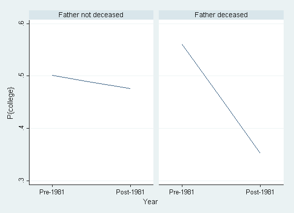
Table 8.2 on page 157, labeled “(First Diff)”. (Note this
replicates the last regression model.)
svy if fatherdec==1 : regress coll offer
(running regress on estimation sample)

Survey: Linear regression

Number of strata   =         1                  Number of obs      =       191
Number of PSUs     =       172                  Population size    =  51656801
                                                Design df          =       171
                                                F(   1,    171)    =      4.96
                                                Prob > F           =    0.0272
                                                R-squared          =    0.0358

------------------------------------------------------------------------------
             |             Linearized
        coll |      Coef.   Std. Err.      t    P>|t|     [95% Conf. Interval]
-------------+----------------------------------------------------------------
       offer |   .2082378   .0935031     2.23   0.027     .0236689    .3928067
       _cons |   .3522178   .0814687     4.32   0.000      .191404    .5130317
------------------------------------------------------------------------------
Table 8.2 on page 157, labeled “(Second Diff)”.
svy if fatherdec==0 : regress coll offer
(running regress on estimation sample)

Survey: Linear regression

Number of strata   =         1                Number of obs      =        3795
Number of PSUs     =      2984                Population size    =  1251276567
                                              Design df          =        2983
                                              F(   1,   2983)    =        1.50
                                              Prob > F           =      0.2214
                                              R-squared          =      0.0006

------------------------------------------------------------------------------
             |             Linearized
        coll |      Coef.   Std. Err.      t    P>|t|     [95% Conf. Interval]
-------------+----------------------------------------------------------------
       offer |   .0260081   .0212645     1.22   0.221    -.0156865    .0677026
       _cons |   .4756935   .0188651    25.22   0.000     .4387037    .5126834
------------------------------------------------------------------------------
Table 8.4 on page 161.
svy: regress coll offer fatherdec offerxfatherdec
(running regress on estimation sample)

Survey: Linear regression

Number of strata   =         1                Number of obs      =        3986
Number of PSUs     =      3123                Population size    =  1302933368
                                              Design df          =        3122
                                              F(   3,   3120)    =        2.19
                                              Prob > F           =      0.0875
                                              R-squared          =      0.0020

------------------------------------------------------------------------------
             |             Linearized
        coll |      Coef.   Std. Err.      t    P>|t|     [95% Conf. Interval]
-------------+----------------------------------------------------------------
       offer |   .0260081   .0212643     1.22   0.221    -.0156854    .0677016
   fatherdec |  -.1234757   .0834251    -1.48   0.139    -.2870493    .0400979
offerxfath~c |   .1822297    .095841     1.90   0.057    -.0056881    .3701475
       _cons |   .4756935   .0188649    25.22   0.000     .4387046    .5126825
------------------------------------------------------------------------------
The “first difference” for cases where the father is not deceased shown in
Table 8.2 can be seen here as the coefficient for offer. The term for the
interaction (offerxfatherdec) is the “second difference.” The syntax
below calculates the “first difference” for cases where the father is deceased.
lincom offer + offerxfatherdec
 ( 1)  offer + offerxfatherdec = 0

------------------------------------------------------------------------------
        coll |      Coef.   Std. Err.      t    P>|t|     [95% Conf. Interval]
-------------+----------------------------------------------------------------
         (1) |   .2082378   .0932458     2.23   0.026     .0254085    .3910671
------------------------------------------------------------------------------
Table 8.4 on page 161 can
also be reproduced using the factor variable syntax introduced in Stata 11.
svy: regress coll offer##fatherdec

(running regress on estimation sample)

Survey: Linear regression

Number of strata   =         1                Number of obs      =        3986
Number of PSUs     =      3123                Population size    =  1302933368
                                              Design df          =        3122
                                              F(   3,   3120)    =        2.19
                                              Prob > F           =      0.0875
                                              R-squared          =      0.0020

------------------------------------------------------------------------------
             |             Linearized
        coll |      Coef.   Std. Err.      t    P>|t|     [95% Conf. Interval]
-------------+----------------------------------------------------------------
     1.offer |   .0260081   .0212643     1.22   0.221    -.0156854    .0677016
 1.fatherdec |  -.1234757   .0834251    -1.48   0.139    -.2870493    .0400979
             |
       offer#|
   fatherdec |
        1 1  |   .1822297    .095841     1.90   0.057    -.0056881    .3701475
             |
       _cons |   .4756935   .0188649    25.22   0.000     .4387046    .5126825
------------------------------------------------------------------------------


lincom 1.offer + 1.offer#1.father

 ( 1)  1.offer + 1.offer#1.fatherdec = 0

------------------------------------------------------------------------------
        coll |      Coef.   Std. Err.      t    P>|t|     [95% Conf. Interval]
-------------+----------------------------------------------------------------
         (1) |   .2082378   .0932458     2.23   0.026     .0254085    .3910671
------------------------------------------------------------------------------