The data set used in this chapter is popular.dta. The programs we use
in this chapter are gllamm and gllapred. You can find the programs and download
them by issuing command search gllamm and search gllapred (see
How can I use
the search command to search for programs and get additional help? for
more information about using search). For
more information see http://www.gllamm.org .
Table 2.1 on page 17.
Part1: Intercept only. (M0). The deviance is obtained by multiplying the log likelihood by -2.
use https://stats.idre.ucla.edu/stat/stata/examples/mlm_ma_hox/popular.dta, clear

gllamm popular, i(school) adapt

number of level 1 units = 2000
number of level 2 units = 100
Condition Number = 5.8576802
gllamm model
log likelihood = -2556.3612
------------------------------------------------------------------------------
     popular |      Coef.   Std. Err.      z    P>|z|     [95% Conf. Interval]
-------------+----------------------------------------------------------------
       _cons |   5.307604   .0950217    55.86   0.000     5.121365    5.493843
------------------------------------------------------------------------------
Variance at level 1
-----------------------------------------------------------------------------
.63867681 (.02072164)
Variances and covariances of random effects
-----------------------------------------------------------------------------
***level 2 (school)
    var(1): .87068762 (.12771943)
-----------------------------------------------------------------------------

di 2*2556.3612
5112.7224
Part 2: The variable sex is included as a random effect and teacher
experience (texp) as fixed effect (M1).
eq sch_s: sex
gen cons = 1
eq sch_c: cons
gllamm popular texp sex, i(school) adapt nrf(2) eq(sch_c sch_s)
number of level 1 units = 2000
number of level 2 units = 100
Condition Number = 40.498391
gllamm model
log likelihood = -2130.5659
------------------------------------------------------------------------------
     popular |      Coef.   Std. Err.      z    P>|z|     [95% Conf. Interval]
-------------+----------------------------------------------------------------
        texp |   .1084215   .0106385    10.19   0.000     .0875704    .1292726
         sex |   .8432452   .0587151    14.36   0.000     .7281656    .9583247
       _cons |   3.339099   .1651731    20.22   0.000     3.015366    3.662832
------------------------------------------------------------------------------
Variance at level 1
-----------------------------------------------------------------------------
.39241954 (.0130915)
Variances and covariances of random effects
-----------------------------------------------------------------------------
***level 2 (school)
    var(1): .40328261 (.06227253)
    cov(1,2): .02171346 (.04195842) cor(1,2): .06576171
    var(2): .27033508 (.04961092)
-----------------------------------------------------------------------------
Table 2.2 on page 20.
Part 1: Same as the last model appeared in table 2.1.Part 2: Cross-level interaction of variable sex and texp
is included. Notice this model takes very LONG time to run.
gen gxt = sex*texp
eq sch_s: sex
gen cons = 1
eq sch_c: cons
gllamm popular texp sex gxt, i(school) adapt nrf(2) eq(sch_c sch_s)
number of level 1 units = 2000
number of level 2 units = 100
Condition Number = 45.72526
gllamm model
log likelihood = -2122.9085
------------------------------------------------------------------------------
     popular |      Coef.   Std. Err.      z    P>|z|     [95% Conf. Interval]
-------------+----------------------------------------------------------------
        texp |   .1102169   .0099904    11.03   0.000      .090636    .1297977
         sex |    1.32949    .130912    10.16   0.000     1.072907    1.586073
         gxt |   -.034026   .0083388    -4.08   0.000    -.0503697   -.0176822
       _cons |   3.313841   .1566164    21.16   0.000     3.006879    3.620804
------------------------------------------------------------------------------
Variance at level 1
-----------------------------------------------------------------------------
.39236316 (.01308622)
Variances and covariances of random effects
-----------------------------------------------------------------------------
***level 2 (school)
    var(1): .40543808 (.0627154)
    cov(1,2): .02386608 (.03657119) cor(1,2): .0795611
    var(2): .22194032 (.04304873)
-----------------------------------------------------------------------------
Table 2.3 on page 21.
Part 1: M1 from table 2.2.
Part 2: Standardized variables. We first created standardized
variables: zpopular, zsex and ztexp.
egen zsex = std(sex)
egen ztexp = std(texp)
eq sch_zs: zsex
egen zpop = std(popular)
gllamm zpop ztexp zsex , i(school) adapt nrf(2) eq(sch_c sch_zs)
number of level 1 units = 2000
number of level 2 units = 100
Condition Number = 3.6590204
gllamm model
log likelihood = -1723.1996
------------------------------------------------------------------------------
        zpop |      Coef.   Std. Err.      z    P>|z|     [95% Conf. Interval]
-------------+----------------------------------------------------------------
       ztexp |   .5790798   .0583238     9.93   0.000     .4647672    .6933923
        zsex |   .3438637   .0242194    14.20   0.000     .2963946    .3913328
       _cons |  -.0097627   .0581163    -0.17   0.867    -.1236685    .1041431
------------------------------------------------------------------------------
Variance at level 1
-----------------------------------------------------------------------------
.26115453 (.00870857)
Variances and covariances of random effects
-----------------------------------------------------------------------------
***level 2 (school)
    var(1): .32405547 (.04869577)
    cov(1,2): .05071581 (.01594587) cor(1,2): .42065269
    var(2): .04485594 (.00834557)
-----------------------------------------------------------------------------
Figure 2.1 on page 23 based on model M1 from Table 2.2. After
running M1, command gllapred can be used to generate various predicted
values. Here we use gllapred first to generate the predicted value using
only the fixed part of the equation (xb) and then generate the posterior
means (empirical Bayes predictions) and standard deviations of the random
effects (u). postm1 corresponds to the random effect of
intercept and postm2 corresponds to the random effect of variable
sex. Therefore, the prediction using both the fixed effect and the random
effect will be our new variable linp below. We can then use it to
generate the standardized residuals, which is stdres.
gllapred p, xb
gllapred post, u adapt
gen linp = p + postm1 + postm2*sex
gen linres = popular - linp
egen stdres = std(linres)
qnorm stdres, yline(0) xline(0) msymbol(X)
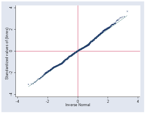
Figure 2.2 on page 24. Based on what we have generated for figure 2.1, we can do
the following:
graph twoway scatter stdres p, yline(0) xlabel(3.5(.9)7.1)
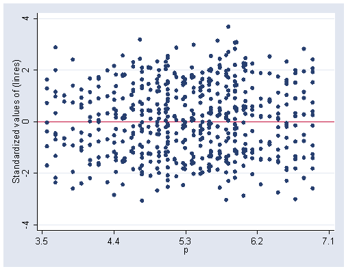
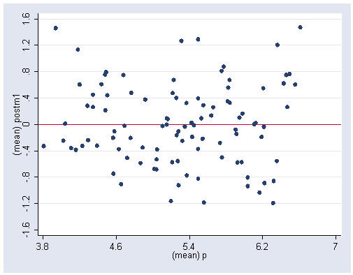
Figure 2.3 on page 24.
collapse (mean) p postm1 posts1 postm2 posts2, by(school)
graph twoway scatter postm1 p, yline(0) ylabel(-1.6(.4) 1.6) xlabel(3.8(.8) 7.0)
. graph twoway scatter postm2 p, yline(0) ylabel(-1.2(.3) 1.2)xlabel(3.8(.8) 7.0)
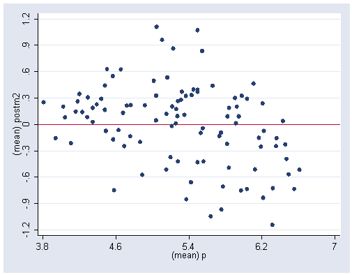
Figure 2.4 on page 25.
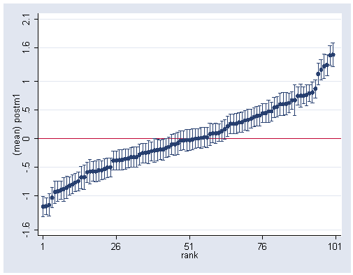
sort postm1
gen rank=_n
serrbar postm1 posts1 rank, yline(0) ylabel(-1.6 -1.0 -.5 0 .5 1 1.6 2.1) xlabel(1(25)101)
drop rank
sort postm2
gen rank=_n
serrbar postm2 posts2 rank, yline(0) ylabel(-1.6 -1.0 -.5 0 .5 1 1.6 2.1) xlabel(1(25)101)
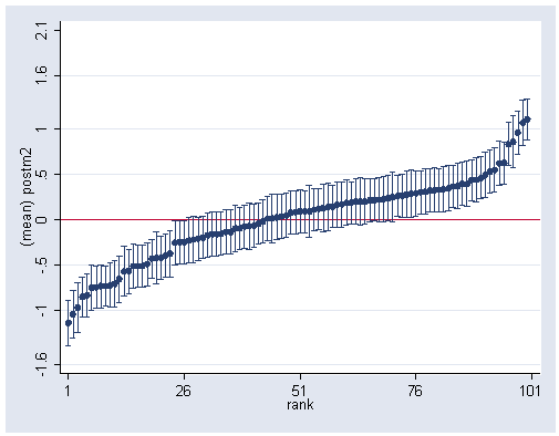
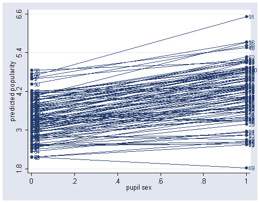
Figure 2.6 on page 28.
gen p26 = linp - .1084215 *texp
label variable p26 "predicted popularity"
sort school sex
graph twoway scatter p26 sex, mlabel(school) connect(L) ylabel(1.8(1.2)6.6)