
Note: the following analysis and results were performed with Stata 14.2
This chapter uses data file gpach5.dta and vocagrwt.dta.
Table 5.1 on page 78.
use https://stats.idre.ucla.edu/stat/stata/examples/mlm_ma_hox/gpach5, clear
keep student sex highgpa gpa time
reshape wide gpa, i(student) j(time)

mat ymat=(1,0,0,0,0,-1\0,1,0,0,0,-1\0,0,1,0,0,-1\0,0,0,1,0,-1\0,0,0,0,1,-1)

manova gpa0 gpa1 gpa2 gpa3 gpa4 gpa5 = sex c.highgpa

                       Number of obs =        200

                       W = Wilks' lambda      L = Lawley-Hotelling trace
                       P = Pillai's trace     R = Roy's largest root

              Source | Statistic        df    F(df1,     df2) =   F   Prob>F
          -----------+-------------------------------------------------------
               Model |W   0.8506         2     12.0    384.0     2.70 0.0017 e
                     |P   0.1534               12.0    386.0     2.67 0.0018 a
                     |L   0.1708               12.0    382.0     2.72 0.0015 a
                     |R   0.1360                6.0    193.0     4.37 0.0004 u
                     |-------------------------------------------------------
            Residual |                 197
          -----------+-------------------------------------------------------
                 sex |W   0.9049         1      6.0    192.0     3.36 0.0036 e
                     |P   0.0951                6.0    192.0     3.36 0.0036 e
                     |L   0.1051                6.0    192.0     3.36 0.0036 e
                     |R   0.1051                6.0    192.0     3.36 0.0036 e
                     |-------------------------------------------------------
             highgpa |W   0.9323         1      6.0    192.0     2.33 0.0343 e
                     |P   0.0677                6.0    192.0     2.33 0.0343 e
                     |L   0.0727                6.0    192.0     2.33 0.0343 e
                     |R   0.0727                6.0    192.0     2.33 0.0343 e
                     |-------------------------------------------------------
            Residual |                 197
          -----------+-------------------------------------------------------
               Total |                 199
          -------------------------------------------------------------------
                       e = exact, a = approximate, u = upper bound on F

*GPA as categorical
mat xcat = (0.5, 0.5,0,1)
manovatest, test(xcat) ytransform(ymat)

 Transformations of the dependent variables
 (1)    gpa0 - gpa5
 (2)    gpa1 - gpa5
 (3)    gpa2 - gpa5
 (4)    gpa3 - gpa5
 (5)    gpa4 - gpa5

 Test constraint
 (1)    .5*0.sex + .5*1.sex + _cons = 0

                       W = Wilks' lambda      L = Lawley-Hotelling trace
                       P = Pillai's trace     R = Roy's largest root

              Source | Statistic        df    F(df1,     df2) =   F   Prob>F
          -----------+-------------------------------------------------------
          manovatest |W   0.8950         1      5.0    193.0     4.53 0.0006 e
                     |P   0.1050                5.0    193.0     4.53 0.0006 e
                     |L   0.1173                5.0    193.0     4.53 0.0006 e
                     |R   0.1173                5.0    193.0     4.53 0.0006 e
                     |-------------------------------------------------------
            Residual |                 197
          -------------------------------------------------------------------
                       e = exact, a = approximate, u = upper bound on F

*linear trend
mat ylin =(-5,-3,-1,1,3,5)
manovatest, test(xcat) ytransform(ylin)

 Transformation of the dependent variables
 (1)    -5*gpa0 - 3*gpa1 - gpa2 + gpa3 + 3*gpa4 + 5*gpa5

 Test constraint
 (1)    .5*0.sex + .5*1.sex + _cons = 0

                       W = Wilks' lambda      L = Lawley-Hotelling trace
                       P = Pillai's trace     R = Roy's largest root

              Source | Statistic        df    F(df1,     df2) =   F   Prob>F
          -----------+-------------------------------------------------------
          manovatest |W   0.9391         1      1.0    197.0    12.77 0.0004 e
                     |P   0.0609                1.0    197.0    12.77 0.0004 e
                     |L   0.0648                1.0    197.0    12.77 0.0004 e
                     |R   0.0648                1.0    197.0    12.77 0.0004 e
                     |-------------------------------------------------------
            Residual |                 197
          -------------------------------------------------------------------
                       e = exact, a = approximate, u = upper bound on F
*gpa*highgpa
manovatest c.highgpa, ytransform(ymat)

 Transformations of the dependent variables
 (1)    gpa0 - gpa5
 (2)    gpa1 - gpa5
 (3)    gpa2 - gpa5
 (4)    gpa3 - gpa5
 (5)    gpa4 - gpa5

                       W = Wilks' lambda      L = Lawley-Hotelling trace
                       P = Pillai's trace     R = Roy's largest root

              Source | Statistic        df    F(df1,     df2) =   F   Prob>F
          -----------+-------------------------------------------------------
             highgpa |W   0.9781         1      5.0    193.0     0.87 0.5053 e
                     |P   0.0219                5.0    193.0     0.87 0.5053 e
                     |L   0.0224                5.0    193.0     0.87 0.5053 e
                     |R   0.0224                5.0    193.0     0.87 0.5053 e
                     |-------------------------------------------------------
            Residual |                 197
          -------------------------------------------------------------------
                       e = exact, a = approximate, u = upper bound on F
*gpa*gender
mat xsex = (1, -1, 0)
manovatest, test(xsex) ytransform(ymat)

 Transformations of the dependent variables
 (1)    gpa0 - gpa5
 (2)    gpa1 - gpa5
 (3)    gpa2 - gpa5
 (4)    gpa3 - gpa5
 (5)    gpa4 - gpa5

 Test constraint
 (1)    0.sex - 1.sex = 0

                       W = Wilks' lambda      L = Lawley-Hotelling trace
                       P = Pillai's trace     R = Roy's largest root

              Source | Statistic        df    F(df1,     df2) =   F   Prob>F
          -----------+-------------------------------------------------------
          manovatest |W   0.9646         1      5.0    193.0     1.42 0.2196 e
                     |P   0.0354                5.0    193.0     1.42 0.2196 e
                     |L   0.0367                5.0    193.0     1.42 0.2196 e
                     |R   0.0367                5.0    193.0     1.42 0.2196 e
                     |-------------------------------------------------------
            Residual |                 197
          -------------------------------------------------------------------
                       e = exact, a = approximate, u = upper bound on F

*test highgpa
mat ym = 1/6*(1,1,1,1,1,1)
manovatest c.highgpa, ytransform(ym)

Transformation of the dependent variables
 (1)    .1666667*gpa0 + .1666667*gpa1 + .1666667*gpa2 + .1666667*gpa3 + .1666667*gpa4 + .1666667*gpa5

                       W = Wilks' lambda      L = Lawley-Hotelling trace
                       P = Pillai's trace     R = Roy's largest root

              Source | Statistic        df    F(df1,     df2) =   F   Prob>F
          -----------+-------------------------------------------------------
             highgpa |W   0.9556         1      1.0    197.0     9.16 0.0028 e
                     |P   0.0444                1.0    197.0     9.16 0.0028 e
                     |L   0.0465                1.0    197.0     9.16 0.0028 e
                     |R   0.0465                1.0    197.0     9.16 0.0028 e
                     |-------------------------------------------------------
            Residual |                 197
          -------------------------------------------------------------------
                       e = exact, a = approximate, u = upper bound on F

*test sex
manovatest, test(xsex) ytransform(ym)

 Transformation of the dependent variables
 (1)    .1666667*gpa0 + .1666667*gpa1 + .1666667*gpa2 + .1666667*gpa3 + .1666667*gpa4 + .1666667*gpa5

 Test constraint
 (1)    0.sex - 1.sex = 0

                       W = Wilks' lambda      L = Lawley-Hotelling trace
                       P = Pillai's trace     R = Roy's largest root

              Source | Statistic        df    F(df1,     df2) =   F   Prob>F
          -----------+-------------------------------------------------------
          manovatest |W   0.9147         1      1.0    197.0    18.37 0.0000 e
                     |P   0.0853                1.0    197.0    18.37 0.0000 e
                     |L   0.0933                1.0    197.0    18.37 0.0000 e
                     |R   0.0933                1.0    197.0    18.37 0.0000 e
                     |-------------------------------------------------------
            Residual |                 197
          -------------------------------------------------------------------
                       e = exact, a = approximate, u = upper bound on F
Table 5.2 on page 79.
use https://stats.idre.ucla.edu/stat/stata/examples/mlm_ma_hox/gpach5, clear
collapse (mean) gpa, by(time sex)
table sex time, contents(mean gpa) col row format(%3.1f)
-----------------------------------------------------------
          |                      time
      sex |     0      1      2      3      4      5  Total
----------+------------------------------------------------
        0 |   2.6    2.7    2.7    2.8    2.9    3.0    2.8
        1 |   2.6    2.8    2.9    3.0    3.1    3.2    2.9
          |
    Total |   2.6    2.7    2.8    2.9    3.0    3.1    2.9
-----------------------------------------------------------
Figure 5.3 on page 80.
use https://stats.idre.ucla.edu/stat/stata/examples/mlm_ma_hox/gpach5, clear
histogram gpa, normal frequency width(.25) start(1.625) xlabel(1.75(.25)4)
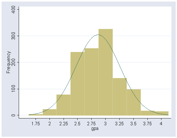
Table 5.3 on page 81.
Part 1: Null model.
use https://stats.idre.ucla.edu/stat/stata/examples/mlm_ma_hox/gpach5, clear
mixed gpa ||student:, var ml

Performing EM optimization:

Performing gradient-based optimization:

Iteration 0:   log likelihood = -456.72811
Iteration 1:   log likelihood = -456.72811

Computing standard errors:

Mixed-effects ML regression                     Number of obs      =      1200
Group variable: student                         Number of groups   =       200

                                                Obs per group: min =         6
                                                               avg =       6.0
                                                               max =         6


                                                Wald chi2(0)       =         .
Log likelihood = -456.72811                     Prob > chi2        =         .

------------------------------------------------------------------------------
         gpa |      Coef.   Std. Err.      z    P>|z|     [95% Conf. Interval]
-------------+----------------------------------------------------------------
       _cons |      2.865   .0191093   149.93   0.000     2.827546    2.902454
------------------------------------------------------------------------------

------------------------------------------------------------------------------
  Random-effects Parameters  |   Estimate   Std. Err.     [95% Conf. Interval]
-----------------------------+------------------------------------------------
student: Identity            |
                  var(_cons) |   .0567683   .0073395      .0440612    .0731402
-----------------------------+------------------------------------------------
               var(Residual) |     .09759   .0043644      .0894002    .1065301
------------------------------------------------------------------------------
LR test vs. linear regression: chibar2(01) =   249.82 Prob >= chibar2 = 0.0000


estat ic

Akaike's information criterion and Bayesian information criterion

-----------------------------------------------------------------------------
       Model |        Obs  ll(null)  ll(model)      df         AIC        BIC
-------------+---------------------------------------------------------------
           . |      1,200         .  -456.7281       3    919.4562   934.7265
-----------------------------------------------------------------------------
Part 2: With additional variable time.
mixed gpa time ||student:, var ml

Performing EM optimization:

Performing gradient-based optimization:

Iteration 0:   log likelihood = -196.82458
Iteration 1:   log likelihood = -196.82458

Computing standard errors:

Mixed-effects ML regression                     Number of obs      =      1200
Group variable: student                         Number of groups   =       200

                                                Obs per group: min =         6
                                                               avg =       6.0
                                                               max =         6


                                                Wald chi2(1)       =    681.70
Log likelihood = -196.82458                     Prob > chi2        =    0.0000

------------------------------------------------------------------------------
         gpa |      Coef.   Std. Err.      z    P>|z|     [95% Conf. Interval]
-------------+----------------------------------------------------------------
        time |   .1063143   .0040719    26.11   0.000     .0983336     .114295
       _cons |   2.599214   .0216516   120.05   0.000     2.556778    2.641651
------------------------------------------------------------------------------

------------------------------------------------------------------------------
  Random-effects Parameters  |   Estimate   Std. Err.     [95% Conf. Interval]
-----------------------------+------------------------------------------------
student: Identity            |
                  var(_cons) |   .0633616   .0073161       .050529    .0794532
-----------------------------+------------------------------------------------
               var(Residual) |   .0580305   .0025952      .0531605    .0633465
------------------------------------------------------------------------------
LR test vs. linear regression: chibar2(01) =   481.33 Prob >= chibar2 = 0.0000


estat ic

------------------------------------------------------------------------------
       Model |    Obs    ll(null)   ll(model)     df          AIC         BIC
-------------+----------------------------------------------------------------
           . |   1200           .   -196.8246      4     401.6492    422.0095
------------------------------------------------------------------------------
Part 3: The variable job is added.
mixed gpa time job ||student:, var ml

Performing EM optimization:

Performing gradient-based optimization:

Iteration 0:   log likelihood =  -160.1304
Iteration 1:   log likelihood =  -160.1304

Computing standard errors:

Mixed-effects ML regression                     Number of obs      =      1200
Group variable: student                         Number of groups   =       200

                                                Obs per group: min =         6
                                                               avg =       6.0
                                                               max =         6


                                                Wald chi2(2)       =    788.20
Log likelihood =  -160.1304                     Prob > chi2        =    0.0000

------------------------------------------------------------------------------
         gpa |      Coef.   Std. Err.      z    P>|z|     [95% Conf. Interval]
-------------+----------------------------------------------------------------
        time |    .103166   .0040021    25.78   0.000     .0953219      .11101
         job |  -.1608636    .018356    -8.76   0.000    -.1968408   -.1248864
       _cons |   2.945837    .044462    66.26   0.000     2.858693    3.032981
------------------------------------------------------------------------------

------------------------------------------------------------------------------
  Random-effects Parameters  |   Estimate   Std. Err.     [95% Conf. Interval]
-----------------------------+------------------------------------------------
student: Identity            |
                  var(_cons) |   .0533597   .0063712      .0422258    .0674291
-----------------------------+------------------------------------------------
               var(Residual) |   .0556077    .002494      .0509282    .0607171
------------------------------------------------------------------------------
LR test vs. linear regression: chibar2(01) =   388.27 Prob >= chibar2 = 0.0000

estat ic

Akaike's information criterion and Bayesian information criterion

-----------------------------------------------------------------------------
       Model |        Obs  ll(null)  ll(model)      df         AIC        BIC
-------------+---------------------------------------------------------------
           . |      1,200         .  -160.1304       5    330.2608   355.7112
-----------------------------------------------------------------------------
               Note: N=Obs used in calculating BIC; see [R] BIC note.
Part 4: The variable highgpa and sex are added to the model.
mixed gpa time job highgpa sex ||student:, var ml

Performing EM optimization:

Performing gradient-based optimization:

Iteration 0:   log likelihood = -147.27246
Iteration 1:   log likelihood = -147.27246

Computing standard errors:

Mixed-effects ML regression                     Number of obs      =      1200
Group variable: student                         Number of groups   =       200

                                                Obs per group: min =         6
                                                               avg =       6.0
                                                               max =         6


                                                Wald chi2(4)       =    820.13
Log likelihood = -147.27246                     Prob > chi2        =    0.0000

------------------------------------------------------------------------------
         gpa |      Coef.   Std. Err.      z    P>|z|     [95% Conf. Interval]
-------------+----------------------------------------------------------------
        time |   .1031482   .0040024    25.77   0.000     .0953037    .1109926
         job |  -.1617732   .0183036    -8.84   0.000    -.1976476   -.1258988
     highgpa |   .0858379   .0279769     3.07   0.002     .0310042    .1406717
         sex |   .1483967   .0333128     4.45   0.000     .0831048    .2136886
       _cons |   2.613448   .0982039    26.61   0.000     2.420972    2.805924
------------------------------------------------------------------------------

------------------------------------------------------------------------------
  Random-effects Parameters  |   Estimate   Std. Err.     [95% Conf. Interval]
-----------------------------+------------------------------------------------
student: Identity            |
                  var(_cons) |   .0457555   .0056063      .0359872    .0581754
-----------------------------+------------------------------------------------
               var(Residual) |    .055617   .0024948      .0509361    .0607281
------------------------------------------------------------------------------
LR test vs. linear regression: chibar2(01) =   333.27 Prob >= chibar2 = 0.0000


estat ic

Akaike's information criterion and Bayesian information criterion

-----------------------------------------------------------------------------
       Model |        Obs  ll(null)  ll(model)      df         AIC        BIC
-------------+---------------------------------------------------------------
           . |      1,200         .  -147.2725       7    308.5449   344.1755
-----------------------------------------------------------------------------
               Note: N=Obs used in calculating BIC; see [R] BIC note.
Table 5.4 on page 83.
Part 1: The variable time is included as a random effect.
mixed gpa time job highgpa sex ||student: time, var ml cov(un)

Performing EM optimization:

Performing gradient-based optimization:

Iteration 0:   log likelihood = -90.102483
Iteration 1:   log likelihood = -90.102468
Iteration 2:   log likelihood = -90.102468

Computing standard errors:

Mixed-effects ML regression                     Number of obs      =      1200
Group variable: student                         Number of groups   =       200

                                                Obs per group: min =         6
                                                               avg =       6.0
                                                               max =         6


                                                Wald chi2(4)       =    431.48
Log likelihood = -90.102468                     Prob > chi2        =    0.0000

------------------------------------------------------------------------------
         gpa |      Coef.   Std. Err.      z    P>|z|     [95% Conf. Interval]
-------------+----------------------------------------------------------------
        time |   .1039731   .0056223    18.49   0.000     .0929537    .1149925
         job |  -.1196211   .0174584    -6.85   0.000    -.1538388   -.0854033
     highgpa |   .0898354   .0264746     3.39   0.001     .0379462    .1417246
         sex |   .1167606   .0315324     3.70   0.000     .0549583     .178563
       _cons |   2.527287   .0926005    27.29   0.000     2.345793     2.70878
------------------------------------------------------------------------------

------------------------------------------------------------------------------
  Random-effects Parameters  |   Estimate   Std. Err.     [95% Conf. Interval]
-----------------------------+------------------------------------------------
student: Unstructured        |
                   var(time) |   .0039121   .0006455       .002831    .0054059
                  var(_cons) |   .0389692   .0062212      .0284991    .0532858
             cov(time,_cons) |  -.0025635   .0015582     -.0056175    .0004905
-----------------------------+------------------------------------------------
               var(Residual) |   .0417646   .0020993      .0378462    .0460887
------------------------------------------------------------------------------
LR test vs. linear regression:       chi2(3) =   447.61   Prob > chi2 = 0.0000

Note: LR test is conservative and provided only for reference

estat ic

Akaike's information criterion and Bayesian information criterion

-----------------------------------------------------------------------------
       Model |        Obs  ll(null)  ll(model)      df         AIC        BIC
-------------+---------------------------------------------------------------
           . |      1,200         .  -90.10247       9    198.2049   244.0156
-----------------------------------------------------------------------------
               Note: N=Obs used in calculating BIC; see [R] BIC note.
Part 2: Cross level interaction of variable time and sex
is included. We first created the interaction term.
gen sxtime= sex*time
mixed gpa time job highgpa sex sxtime ||student: time, var ml cov(un)

Performing EM optimization:

Performing gradient-based optimization:

Iteration 0:   log likelihood = -86.602037
Iteration 1:   log likelihood = -86.602002
Iteration 2:   log likelihood = -86.602002

Computing standard errors:

Mixed-effects ML regression                     Number of obs      =      1200
Group variable: student                         Number of groups   =       200

                                                Obs per group: min =         6
                                                               avg =       6.0
                                                               max =         6


                                                Wald chi2(5)       =    452.34
Log likelihood = -86.602002                     Prob > chi2        =    0.0000

------------------------------------------------------------------------------
         gpa |      Coef.   Std. Err.      z    P>|z|     [95% Conf. Interval]
-------------+----------------------------------------------------------------
        time |   .0884798   .0080081    11.05   0.000     .0727841    .1041754
         job |  -.1206129   .0174249    -6.92   0.000    -.1547651   -.0864606
     highgpa |   .0898068   .0264668     3.39   0.001     .0379327    .1416808
         sex |   .0767958   .0348988     2.20   0.028     .0083954    .1451962
      sxtime |   .0294742   .0110399     2.67   0.008     .0078363     .051112
       _cons |   2.550491   .0928935    27.46   0.000     2.368423    2.732559
------------------------------------------------------------------------------

------------------------------------------------------------------------------
  Random-effects Parameters  |   Estimate   Std. Err.     [95% Conf. Interval]
-----------------------------+------------------------------------------------
student: Unstructured        |
                   var(time) |   .0036912   .0006242      .0026499    .0051418
                  var(_cons) |   .0385556   .0061494      .0282049    .0527048
             cov(time,_cons) |   -.002273   .0015061     -.0052248    .0006789
-----------------------------+------------------------------------------------
               var(Residual) |   .0417767   .0021004      .0378562    .0461031
------------------------------------------------------------------------------
LR test vs. linear regression:       chi2(3) =   446.52   Prob > chi2 = 0.0000

Note: LR test is conservative and provided only for reference

estat ic

------------------------------------------------------------------------------
       Model |    Obs    ll(null)   ll(model)     df          AIC         BIC
-------------+----------------------------------------------------------------
           . |   1200           .     -86.602     10      193.204    244.1048
------------------------------------------------------------------------------
Figure 5.4 on page 84 based on the previous model.
gen p = 2.55 + .088*time + .0768*sex + .029*sxtime
sort sex time
label variable p "Predicted GPA"
twoway scatter p time, connect(L) ylabel(2.5(.1)3.3)
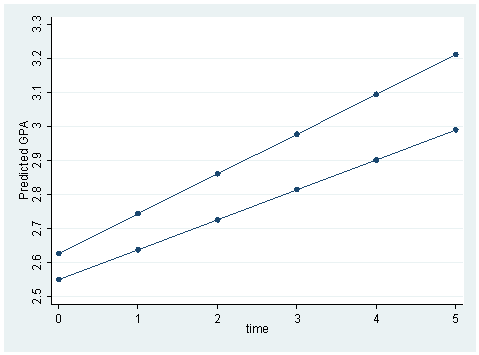
Table 5.5 on page 85.
tab time
       time |      Freq.     Percent        Cum.
------------+-----------------------------------
          0 |        200       16.67       16.67
          1 |        200       16.67       33.33
          2 |        200       16.67       50.00
          3 |        200       16.67       66.67
          4 |        200       16.67       83.33
          5 |        200       16.67      100.00
------------+-----------------------------------
      Total |      1,200      100.00
Part 1: 1st occasion = 0, same as the first part of Table 5.4.
mixed gpa time job highgpa sex ||student: time, var ml cov(un)


------------------------------------------------------------------------------
         gpa |      Coef.   Std. Err.      z    P>|z|     [95% Conf. Interval]
-------------+----------------------------------------------------------------
        time |   .1039731   .0056223    18.49   0.000     .0929537    .1149925
         job |  -.1196211   .0174584    -6.85   0.000    -.1538388   -.0854033
     highgpa |   .0898354   .0264746     3.39   0.001     .0379462    .1417246
         sex |   .1167606   .0315324     3.70   0.000     .0549583     .178563
       _cons |   2.527287   .0926005    27.29   0.000     2.345793     2.70878
------------------------------------------------------------------------------

------------------------------------------------------------------------------
  Random-effects Parameters  |   Estimate   Std. Err.     [95% Conf. Interval]
-----------------------------+------------------------------------------------
student: Unstructured        |
                   var(time) |   .0039121   .0006455       .002831    .0054059
                  var(_cons) |   .0389692   .0062212      .0284991    .0532858
             cov(time,_cons) |  -.0025635   .0015582     -.0056175    .0004905
-----------------------------+------------------------------------------------
               var(Residual) |   .0417646   .0020993      .0378462    .0460887
------------------------------------------------------------------------------
LR test vs. linear regression:       chi2(3) =   447.61   Prob > chi2 = 0.0000
Part 2: The variable time has been recoded as -5, …,-1, 0, …with the
last occasion coded as zero. We first recode variable time into time1.
gen time1 = time -5
mixed gpa time1 job highgpa sex ||student: time1, var ml cov(un)
Performing EM optimization:

Performing gradient-based optimization:

Iteration 0:   log likelihood = -90.102485
Iteration 1:   log likelihood = -90.102468
Iteration 2:   log likelihood = -90.102468

Computing standard errors:

Mixed-effects ML regression                     Number of obs      =      1200
Group variable: student                         Number of groups   =       200

                                                Obs per group: min =         6
                                                               avg =       6.0
                                                               max =         6


                                                Wald chi2(4)       =    431.48
Log likelihood = -90.102468                     Prob > chi2        =    0.0000

------------------------------------------------------------------------------
         gpa |      Coef.   Std. Err.      z    P>|z|     [95% Conf. Interval]
-------------+----------------------------------------------------------------
       time1 |   .1039731   .0056223    18.49   0.000     .0929537    .1149926
         job |  -.1196211   .0174584    -6.85   0.000    -.1538388   -.0854033
     highgpa |   .0898354   .0264746     3.39   0.001     .0379462    .1417246
         sex |   .1167606   .0315324     3.70   0.000     .0549583     .178563
       _cons |   3.047152   .0938291    32.48   0.000      2.86325    3.231054
------------------------------------------------------------------------------

------------------------------------------------------------------------------
  Random-effects Parameters  |   Estimate   Std. Err.     [95% Conf. Interval]
-----------------------------+------------------------------------------------
student: Unstructured        |
                  var(time1) |   .0039121   .0006455       .002831    .0054059
                  var(_cons) |   .1111359   .0137347      .0872286    .1415956
            cov(time1,_cons) |   .0169968    .002676      .0117519    .0222417
-----------------------------+------------------------------------------------
               var(Residual) |   .0417646   .0020993      .0378462    .0460887
------------------------------------------------------------------------------
LR test vs. linear regression:       chi2(3) =   447.61   Prob > chi2 = 0.0000
Part 3: The variable time is recoded centered around its mean and
is included as a fixed effect.
gen timec = time - 2.5
mixed gpa timec job highgpa sex ||student: timec, var ml cov(un)

Performing EM optimization:

Performing gradient-based optimization:

Iteration 0:   log likelihood = -90.102706
Iteration 1:   log likelihood = -90.102468
Iteration 2:   log likelihood = -90.102468

Computing standard errors:

Mixed-effects ML regression                     Number of obs      =      1200
Group variable: student                         Number of groups   =       200

                                                Obs per group: min =         6
                                                               avg =       6.0
                                                               max =         6


                                                Wald chi2(4)       =    431.48
Log likelihood = -90.102468                     Prob > chi2        =    0.0000

------------------------------------------------------------------------------
         gpa |      Coef.   Std. Err.      z    P>|z|     [95% Conf. Interval]
-------------+----------------------------------------------------------------
       timec |   .1039731   .0056223    18.49   0.000     .0929537    .1149926
         job |  -.1196211   .0174584    -6.85   0.000    -.1538388   -.0854033
     highgpa |   .0898354   .0264746     3.39   0.001     .0379462    .1417246
         sex |   .1167606   .0315324     3.70   0.000     .0549583     .178563
       _cons |   2.787219    .092151    30.25   0.000     2.606607    2.967832
------------------------------------------------------------------------------

------------------------------------------------------------------------------
  Random-effects Parameters  |   Estimate   Std. Err.     [95% Conf. Interval]
-----------------------------+------------------------------------------------
student: Unstructured        |
                  var(timec) |   .0039121   .0006455       .002831    .0054059
                  var(_cons) |   .0506022   .0058846      .0402885     .063556
            cov(timec,_cons) |   .0072167   .0014799      .0043162    .0101172
-----------------------------+------------------------------------------------
               var(Residual) |   .0417646   .0020993      .0378462    .0460887
------------------------------------------------------------------------------
LR test vs. linear regression:       chi2(3) =   447.61   Prob > chi2 = 0.0000
Table 5.6 using data file vocagrwt.dta.
use https://stats.idre.ucla.edu/stat/stata/examples/mlm_ma_hox/vocagrwt, clear

table age, contents (count child)

----------------------
age in    |
months    |   N(child)
----------+-----------
       12 |         22
       14 |          5
       16 |         22
       18 |         11
       20 |         22
       22 |         11
       24 |         22
       26 |         11
----------------------
Table 5.7 on page 89. We have to recode the variable study as follows.
Part 1: Intercept only model.
gen study1 = study - .5
mixed vocab study1 ||child:, var ml cov(un)

Note: single-variable random-effects specification; covariance structure set to
      identity

Performing EM optimization:

Performing gradient-based optimization:

Iteration 0:   log likelihood = -834.45287
Iteration 1:   log likelihood = -834.45002
Iteration 2:   log likelihood = -834.45001

Computing standard errors:

Mixed-effects ML regression                     Number of obs      =       126
Group variable: child                           Number of groups   =        22

                                                Obs per group: min =         4
                                                               avg =       5.7
                                                               max =         8


                                                Wald chi2(1)       =      8.08
Log likelihood = -834.45001                     Prob > chi2        =    0.0045

------------------------------------------------------------------------------
       vocab |      Coef.   Std. Err.      z    P>|z|     [95% Conf. Interval]
-------------+----------------------------------------------------------------
      study1 |   -110.912    39.0169    -2.84   0.004    -187.3838   -34.44031
       _cons |   132.0697   19.50845     6.77   0.000     93.83379    170.3055
------------------------------------------------------------------------------

------------------------------------------------------------------------------
  Random-effects Parameters  |   Estimate   Std. Err.     [95% Conf. Interval]
-----------------------------+------------------------------------------------
child: Identity              |
                  var(_cons) |   2400.597    2148.08      415.5804    13867.03
-----------------------------+------------------------------------------------
               var(Residual) |   31075.49   4201.565      23841.37    40504.64
------------------------------------------------------------------------------
LR test vs. linear regression: chibar2(01) =     1.94 Prob >= chibar2 = 0.0821
Part 2: The variable age is grand mean centered and is included as
a fixed effect.
sum age

    Variable |       Obs        Mean    Std. Dev.       Min        Max
-------------+--------------------------------------------------------
         age |       126    18.88889    4.578598         12         26

gen agec=age-r(mean)
mixed vocab study1 agec ||child:, var ml cov(un)

Note: single-variable random-effects specification; covariance structure set to
      identity

Performing EM optimization:

Performing gradient-based optimization:

Iteration 0:   log likelihood = -775.46764
Iteration 1:   log likelihood = -775.46764

Computing standard errors:

Mixed-effects ML regression                     Number of obs      =       126
Group variable: child                           Number of groups   =        22

                                                Obs per group: min =         4
                                                               avg =       5.7
                                                               max =         8


                                                Wald chi2(2)       =    225.19
Log likelihood = -775.46764                     Prob > chi2        =    0.0000

------------------------------------------------------------------------------
       vocab |      Coef.   Std. Err.      z    P>|z|     [95% Conf. Interval]
-------------+----------------------------------------------------------------
      study1 |  -69.79256   35.47381    -1.97   0.049    -139.3199   -.2651797
        agec |   29.55533   2.013816    14.68   0.000     25.60832    33.50233
       _cons |   137.7813   17.68648     7.79   0.000     103.1165    172.4462
------------------------------------------------------------------------------

------------------------------------------------------------------------------
  Random-effects Parameters  |   Estimate   Std. Err.     [95% Conf. Interval]
-----------------------------+------------------------------------------------
child: Identity              |
                  var(_cons) |   4882.778   1937.101      2243.765    10625.68
-----------------------------+------------------------------------------------
               var(Residual) |   10377.41   1421.189      7934.449    13572.54
------------------------------------------------------------------------------
LR test vs. linear regression: chibar2(01) =    26.44 Prob >= chibar2 = 0.0000
Part 3: The squared term of agec is included as a fixed effect.
gen agec2 = agec*agec
mixed vocab study1 agec agec2 ||child:, var ml cov(un)

Note: single-variable random-effects specification; covariance structure set to
      identity

Performing EM optimization:

Performing gradient-based optimization:

Iteration 0:   log likelihood = -759.74092
Iteration 1:   log likelihood = -759.74092

Computing standard errors:

Mixed-effects ML regression                     Number of obs      =       126
Group variable: child                           Number of groups   =        22

                                                Obs per group: min =         4
                                                               avg =       5.7
                                                               max =         8


                                                Wald chi2(3)       =    336.38
Log likelihood = -759.74092                     Prob > chi2        =    0.0000

------------------------------------------------------------------------------
       vocab |      Coef.   Std. Err.      z    P>|z|     [95% Conf. Interval]
-------------+----------------------------------------------------------------
      study1 |  -68.25089   34.85923    -1.96   0.050    -136.5737    .0719371
        agec |   30.62189   1.746006    17.54   0.000     27.19978    34.04399
       agec2 |   2.557313    .422708     6.05   0.000     1.728821    3.385806
       _cons |   84.79167   19.46981     4.36   0.000     46.63154    122.9518
------------------------------------------------------------------------------

------------------------------------------------------------------------------
  Random-effects Parameters  |   Estimate   Std. Err.     [95% Conf. Interval]
-----------------------------+------------------------------------------------
child: Identity              |
                  var(_cons) |   5166.262   1902.714      2510.049    10633.36
-----------------------------+------------------------------------------------
               var(Residual) |   7721.242   1060.154      5899.485    10105.55
------------------------------------------------------------------------------
LR test vs. linear regression: chibar2(01) =    38.85 Prob >= chibar2 = 0.0000
Part 4: The centered variable agec is included as a random effect.
mixed vocab study1 agec agec2 || child: agec, var ml cov(un)

(note Stata 14.2 results in Hessian not negative semidefinite error)

Performing EM optimization:

Performing gradient-based optimization:

Iteration 0:   log likelihood = -651.93737
Iteration 1:   log likelihood = -651.40036
Iteration 2:   log likelihood = -651.37911
Iteration 3:   log likelihood = -651.37642
Iteration 4:   log likelihood = -651.37628
Iteration 5:   log likelihood = -651.37626

Computing standard errors:

Mixed-effects ML regression                     Number of obs      =       126
Group variable: child                           Number of groups   =        22

                                                Obs per group: min =         4
                                                               avg =       5.7
                                                               max =         8


                                                Wald chi2(3)       =    288.74
Log likelihood = -651.37626                     Prob > chi2        =    0.0000

------------------------------------------------------------------------------
       vocab |      Coef.   Std. Err.      z    P>|z|     [95% Conf. Interval]
-------------+----------------------------------------------------------------
      study1 |  -4.971305   8.003023    -0.62   0.534    -20.65694    10.71433
        agec |   28.13162   3.399128     8.28   0.000     21.46945    34.79379
       agec2 |   2.175139   .1454073    14.96   0.000     1.890146    2.460132
       _cons |     87.982   17.52353     5.02   0.000     53.63651    122.3275
------------------------------------------------------------------------------

------------------------------------------------------------------------------
  Random-effects Parameters  |   Estimate   Std. Err.     [95% Conf. Interval]
-----------------------------+------------------------------------------------
child: Unstructured          |
                   var(agec) |   245.7646   76.12805      133.9218    451.0114
                  var(_cons) |   6399.886   1995.074      3473.939    11790.23
             cov(agec,_cons) |   1254.139   384.1707      501.1785      2007.1
-----------------------------+------------------------------------------------
               var(Residual) |   862.6386   119.6392      657.3185    1132.092
------------------------------------------------------------------------------
LR test vs. linear regression:       chi2(3) =   255.58   Prob > chi2 = 0.0000

Note: LR test is conservative and provided only for reference
Table 5.8 on page 91.
Part 1: Intercept only model. This is Part 1 from Table 5.7. We only show the output here.
------------------------------------------------------------------------------
       vocab |      Coef.   Std. Err.      z    P>|z|     [95% Conf. Interval]
-------------+----------------------------------------------------------------
      study1 |   -110.912    39.0169    -2.84   0.004    -187.3838   -34.44031
       _cons |   132.0697   19.50845     6.77   0.000     93.83379    170.3055
------------------------------------------------------------------------------

------------------------------------------------------------------------------
  Random-effects Parameters  |   Estimate   Std. Err.     [95% Conf. Interval]
-----------------------------+------------------------------------------------
child: Identity              |
                  var(_cons) |   2400.597    2148.08      415.5804    13867.03
-----------------------------+------------------------------------------------
               var(Residual) |   31075.49   4201.565      23841.37    40504.64
------------------------------------------------------------------------------
Part 2: The variable age is centered on 12 months and is included
as a fixed effect.
mixed vocab study1 age12 ||child: , var ml cov(un)

Note: single-variable random-effects specification; covariance structure set to
      identity

Performing EM optimization:

Performing gradient-based optimization:

Iteration 0:   log likelihood = -775.46764
Iteration 1:   log likelihood = -775.46764

Computing standard errors:

Mixed-effects ML regression                     Number of obs      =       126
Group variable: child                           Number of groups   =        22

                                                Obs per group: min =         4
                                                               avg =       5.7
                                                               max =         8


                                                Wald chi2(2)       =    225.19
Log likelihood = -775.46764                     Prob > chi2        =    0.0000

------------------------------------------------------------------------------
       vocab |      Coef.   Std. Err.      z    P>|z|     [95% Conf. Interval]
-------------+----------------------------------------------------------------
      study1 |  -69.79256   35.47381    -1.97   0.049    -139.3199   -.2651795
       age12 |   29.55533   2.013816    14.68   0.000     25.60832    33.50233
       _cons |  -65.82204    22.2324    -2.96   0.003    -109.3967   -22.24734
------------------------------------------------------------------------------

------------------------------------------------------------------------------
  Random-effects Parameters  |   Estimate   Std. Err.     [95% Conf. Interval]
-----------------------------+------------------------------------------------
child: Identity              |
                  var(_cons) |   4882.778   1937.101      2243.765    10625.68
-----------------------------+------------------------------------------------
               var(Residual) |   10377.41   1421.189      7934.449    13572.54
------------------------------------------------------------------------------
LR test vs. linear regression: chibar2(01) =    26.44 Prob >= chibar2 = 0.0000

estat ic

Akaike's information criterion and Bayesian information criterion

-----------------------------------------------------------------------------
       Model |        Obs  ll(null)  ll(model)      df         AIC        BIC
-------------+---------------------------------------------------------------
           . |        126         .  -775.4676       5    1560.935   1575.117
-----------------------------------------------------------------------------
               Note: N=Obs used in calculating BIC; see [R] BIC note.
Part 3: The variable age12sq is included as a fixed effect.
mixed vocab study1 age12 age12sq ||child: , var ml cov(un)

Note: single-variable random-effects specification; covariance structure set to
      identity

Performing EM optimization:

Performing gradient-based optimization:

Iteration 0:   log likelihood = -759.74092
Iteration 1:   log likelihood = -759.74092

Computing standard errors:

Mixed-effects ML regression                     Number of obs     =        126
Group variable: child                           Number of groups  =         22

                                                Obs per group:
                                                              min =          4
                                                              avg =        5.7
                                                              max =          8

                                                Wald chi2(3)      =     336.38
Log likelihood = -759.74092                     Prob > chi2       =     0.0000

------------------------------------------------------------------------------
       vocab |      Coef.   Std. Err.      z    P>|z|     [95% Conf. Interval]
-------------+----------------------------------------------------------------
      study1 |  -68.25089   34.85924    -1.96   0.050    -136.5737    .0719587
       age12 |  -4.612211   5.910617    -0.78   0.435    -16.19681    6.972385
     age12sq |   2.557313    .422708     6.05   0.000     1.728821    3.385806
       _cons |  -4.797205   23.22993    -0.21   0.836    -50.32703    40.73262
------------------------------------------------------------------------------

------------------------------------------------------------------------------
  Random-effects Parameters  |   Estimate   Std. Err.     [95% Conf. Interval]
-----------------------------+------------------------------------------------
child: Identity              |
                  var(_cons) |   5166.266   1902.716      2510.051    10633.37
-----------------------------+------------------------------------------------
               var(Residual) |   7721.241   1060.154      5899.485    10105.55
------------------------------------------------------------------------------
LR test vs. linear model: chibar2(01) = 38.85         Prob >= chibar2 = 0.0000

estat ic

Akaike's information criterion and Bayesian information criterion

-----------------------------------------------------------------------------
       Model |        Obs  ll(null)  ll(model)      df         AIC        BIC
-------------+---------------------------------------------------------------
           . |        126         .  -759.7409       6    1531.482     1548.5
-----------------------------------------------------------------------------
               Note: N=Obs used in calculating BIC; see [R] BIC note.
Part 4: The variable age12 is a random effect.
mixed vocab study1 age12 age12sq ||child: age12, var ml cov(un)

(note Stata 14.2 results in Hessian not negative semidefinite error)

Performing EM optimization:

Performing gradient-based optimization:

Iteration 0:   log likelihood =  -652.0315
Iteration 1:   log likelihood = -651.50087
Iteration 2:   log likelihood = -651.40437
Iteration 3:   log likelihood = -651.38281
Iteration 4:   log likelihood = -651.37783
Iteration 5:   log likelihood = -651.37663
Iteration 6:   log likelihood = -651.37632
Iteration 7:   log likelihood = -651.37627
Iteration 8:   log likelihood = -651.37626

Computing standard errors:

Mixed-effects ML regression                     Number of obs      =       126
Group variable: child                           Number of groups   =        22

                                                Obs per group: min =         4
                                                               avg =       5.7
                                                               max =         8


                                                Wald chi2(3)       =    288.73
Log likelihood = -651.37626                     Prob > chi2        =    0.0000

------------------------------------------------------------------------------
       vocab |      Coef.   Std. Err.      z    P>|z|     [95% Conf. Interval]
-------------+----------------------------------------------------------------
      study1 |  -4.975021   8.002868    -0.62   0.534    -20.66035    10.71031
       age12 |  -1.836976   3.891349    -0.47   0.637     -9.46388    5.789927
     age12sq |    2.17514   .1454086    14.96   0.000     1.890144    2.460136
       _cons |  -2.588417   8.341687    -0.31   0.756    -18.93782    13.76099
------------------------------------------------------------------------------

------------------------------------------------------------------------------
  Random-effects Parameters  |   Estimate   Std. Err.     [95% Conf. Interval]
-----------------------------+------------------------------------------------
child: Unstructured          |
                  var(age12) |   245.7569   76.12895      133.9141    451.0091
                  var(_cons) |   784.0285   361.7215       317.409     1936.62
            cov(age12,_cons) |  -438.9538   159.5462     -751.6586   -126.2489
-----------------------------+------------------------------------------------
               var(Residual) |   862.6541   119.6425      657.3286    1132.116
------------------------------------------------------------------------------
LR test vs. linear regression:       chi2(3) =   255.58   Prob > chi2 = 0.0000

Note: LR test is conservative and provided only for reference

estat ic

Akaike's information criterion and Bayesian information criterion

-----------------------------------------------------------------------------
       Model |        Obs  ll(null)  ll(model)      df         AIC        BIC
-------------+---------------------------------------------------------------
           . |        126         .  -779.1681       4    1566.336   1577.681
-----------------------------------------------------------------------------
               Note: N=Obs used in calculating BIC; see [R] BIC note.
Table 5.9 on page 92 is created using HLM. We omit it here.
Table 5.10 on page 101 using the data file gpach5.dta.
use https://stats.idre.ucla.edu/stat/stata/examples/mlm_ma_hox/gpach5, clear
Part 1: The variable time is a fixed effect. We have built the
model at the beginning of this chapter. We will use it here.
mixed gpa time job highgpa sex ||student: , var ml

------------------------------------------------------------------------------
         gpa |      Coef.   Std. Err.      z    P>|z|     [95% Conf. Interval]
-------------+----------------------------------------------------------------
        time |   .1031482   .0040024    25.77   0.000     .0953037    .1109926
         job |  -.1617732   .0183036    -8.84   0.000    -.1976476   -.1258988
     highgpa |   .0858379   .0279769     3.07   0.002     .0310042    .1406717
         sex |   .1483967   .0333128     4.45   0.000     .0831048    .2136886
       _cons |   2.613448   .0982039    26.61   0.000     2.420972    2.805924
------------------------------------------------------------------------------

------------------------------------------------------------------------------
  Random-effects Parameters  |   Estimate   Std. Err.     [95% Conf. Interval]
-----------------------------+------------------------------------------------
student: Identity            |
                  var(_cons) |   .0457555   .0056063      .0359872    .0581754
-----------------------------+------------------------------------------------
               var(Residual) |    .055617   .0024948      .0509361    .0607281
------------------------------------------------------------------------------
LR test vs. linear regression: chibar2(01) =   333.27 Prob >= chibar2 = 0.0000
Part 2: The variable time is included as random effect. This is Part 1 of
table 5.4.
mixed gpa time job highgpa sex ||student: time, var ml cov(un)

------------------------------------------------------------------------------
         gpa |      Coef.   Std. Err.      z    P>|z|     [95% Conf. Interval]
-------------+----------------------------------------------------------------
        time |   .1039731   .0056223    18.49   0.000     .0929537    .1149925
         job |  -.1196211   .0174584    -6.85   0.000    -.1538388   -.0854033
     highgpa |   .0898354   .0264746     3.39   0.001     .0379462    .1417246
         sex |   .1167606   .0315324     3.70   0.000     .0549583     .178563
       _cons |   2.527287   .0926005    27.29   0.000     2.345793     2.70878
------------------------------------------------------------------------------

------------------------------------------------------------------------------
  Random-effects Parameters  |   Estimate   Std. Err.     [95% Conf. Interval]
-----------------------------+------------------------------------------------
student: Unstructured        |
                   var(time) |   .0039121   .0006455       .002831    .0054059
                  var(_cons) |   .0389692   .0062212      .0284991    .0532858
             cov(time,_cons) |  -.0025635   .0015582     -.0056175    .0004905
-----------------------------+------------------------------------------------
               var(Residual) |   .0417646   .0020993      .0378462    .0460887
------------------------------------------------------------------------------
LR test vs. linear regression:       chi2(3) =   447.61   Prob > chi2 = 0.0000

Note: LR test is conservative and provided only for reference
Part 3: The variable time is a fixed effect, MANOVA.