
Multiple regression models often contain interaction terms. This FAQ page
covers the situation in which there are two moderator
variables which jointly influence the regression of the dependent
variable on an independent variable. In other words, a regression
model that has a significant three-way interaction of continuous variables.
If you are new to the topic of interactions of continuous variables, you may
want to start with the FAQ page the discusses the simpler continuous by
continuous two-way interaction,
How can I explain a continuous
by continuous interaction?
Back to the three-way interaction. There are several approaches that one might use to
explain a three-way interaction.
The approach that we will demonstrate is to compute simple slopes, i.e., the
slopes of the dependent variable on the independent variable when the moderator variables are held constant at
different combinations of high and low values. After computing the
simple slopes, we will then compute and test the differences among all
pairs of the slopes.
The method used in this FAQ is adapted from a paper by Dawson and Richter (2004). The
Dawson and Richter method computes the
differences in simple slopes and their standard errors using a number of moderately-complex
formulas. We will take an
easier path and let margins do all of the heavy lifting.
We will begin by looking at the regression equation which includes a three-way
continuous interaction. In the formula, Y is the response variable, X the predictor
(independent) variable with Z and W being the two moderator variables.
Y = b0 + b1X + b2Z + b3W + b4XZ + b5XW + b6ZW + b7XZW
We can reorder the terms into two groups, the first grouping (terms that do not contain X) defines the intercept while the
second grouping (all the terms that contain an X) defines the simple slope.
Y = (b0 + b2Z + b3W + b6ZW) + (b1 + b4Z + b5W + b7ZW)X
Next, we will define high values of Z and W as being one standard deviation above their
respective means and will denote them as Hz and Hw.
The low values will be
defined as one standard deviation below their means and will be as Lz and Lw.
Altogether there are four possible combinations of conditions: 1) HzHw, 2) HzLw,
3) LzHw and 4) LzLw.
Here is the formula for the simple slope for condition 1) when both Z and
W are at their high values. The formulas for the other three conditions are exactly the
same except that the values for Z and W are different.
simple slope 1 = b1 + b4Hz + b5Hw + b7HzHw
We will illustrate the simple slopes process using the dataset hsb2 that has a
statistically significant (barely) three-way continuous interaction. In order to keep
the notation consistent we
will temporarily change the names of the variables; y for the response variable, x
for the independent variable, z for the first moderator, and w for the second
moderator. It is clear from the code below that write is the response variable,
read is the IV and math and science are the moderator variables.
use https://stats.idre.ucla.edu/stat/stata/notes/hsb2, clear

rename write y
rename read x
rename math w
rename science z

regress y c.x##c.z##c.w

      Source |       SS       df       MS              Number of obs =     200
-------------+------------------------------           F(  7,   192) =   26.28
       Model |  8748.54751     7   1249.7925           Prob > F      =  0.0000
    Residual |  9130.32749   192   47.553789           R-squared     =  0.4893
-------------+------------------------------           Adj R-squared =  0.4707
       Total |   17878.875   199   89.843593           Root MSE      =  6.8959

------------------------------------------------------------------------------
           y |      Coef.   Std. Err.      t    P>|t|     [95% Conf. Interval]
-------------+----------------------------------------------------------------
           x |  -3.013849   1.802977    -1.67   0.096    -6.570035    .5423358
           z |  -2.435316   1.757363    -1.39   0.167    -5.901532      1.0309
             |
     c.x#c.z |   .0553139   .0325207     1.70   0.091    -.0088297    .1194576
             |
           w |  -3.228097   1.926393    -1.68   0.095    -7.027708    .5715142
             |
     c.x#c.w |   .0737523    .035898     2.05   0.041     .0029472    .1445575
             |
     c.z#c.w |   .0611136    .035031     1.74   0.083    -.0079813    .1302086
             |
 c.x#c.z#c.w |  -.0012563   .0006277    -2.00   0.047    -.0024944   -.0000182
             |
       _cons |   166.5438   93.12788     1.79   0.075     -17.1413    350.2289
------------------------------------------------------------------------------
Please note that the three-way interaction, xzw, is statistically significant with
a p-value of .047.
We will create four global macros that contain the values
w and z when that are one standard deviation above the mean and one
standard deviation below the mean.
/* determine range of x for graphing */

sum x

    Variable |       Obs        Mean    Std. Dev.       Min        Max
-------------+--------------------------------------------------------
           x |       200       52.23    10.25294         28         76

sum w

    Variable |       Obs        Mean    Std. Dev.       Min        Max
-------------+--------------------------------------------------------
           w |       200      52.645    9.368448         33         75

/* determined high and low values for w */
global Hw=r(mean)+r(sd)
global Lw=r(mean)-r(sd)

sum z

    Variable |       Obs        Mean    Std. Dev.       Min        Max
-------------+--------------------------------------------------------
           z |       200       51.85    9.900891         26         74

/* determine high and low values for z */
global Hz=r(mean)+r(sd)
global Lz=r(mean)-r(sd)
We will use the margins comand to compute the simple slopes for the four
values of w and z. We use the dydx option to obtain the slopes.
Please
note, we have manually annotated the output with the various combinations of w and z in parentheses.
margins, dydx(x) at(w=($Hw $Lw) z=($Hz $Lz)) vsquish

Average marginal effects                          Number of obs   =        200
Model VCE    : OLS

Expression   : Linear prediction, predict()
dy/dx w.r.t. : x

1._at        : z               =    61.75089
               w               =    62.01345
2._at        : z               =    61.75089
               w               =    43.27655
3._at        : z               =    41.94911
               w               =    62.01345
4._at        : z               =    41.94911
               w               =    43.27655

------------------------------------------------------------------------------
             |            Delta-method
             |      dy/dx   Std. Err.      z    P>|z|     [95% Conf. Interval]
-------------+----------------------------------------------------------------
x            |
         _at |
  (HwHz)  1  |    .164556   .0953841     1.73   0.084    -.0223935    .3515054
  (LwHz)  2  |    .236248   .1429934     1.65   0.099    -.0440138    .5165098
  (HwLz)  3  |   .6119673   .1962032     3.12   0.002      .227416    .9965186
  (LwLz)  4  |   .2175364   .1275474     1.71   0.088    -.0324519    .4675248
------------------------------------------------------------------------------
The simple slopes for HwHz, LwHz and LwLz are all fairly similar. However, the slope for Hwlz seems
to be rather different from the other three.
The next step is to graph the slopes along with a scatterplot of the observations. We will use the
margins command again to get the information for plotting. Because we are using linear
regression, we need only two points to define each simple slope regression line. We will
use the x values 20 and 80 which cover more the full range of variable x.
(introduced in Stata 12) command.
margins, at(x=(20 80) w=($Hw $Lw) z=($Hz $Lz)) vsquish

Adjusted predictions                              Number of obs   =        200

Model VCE    : OLS

Expression   : Linear prediction, predict()

1._at        : x               =          20
               z               =    61.75089
               w               =    62.01345
2._at        : x               =          20
               z               =    61.75089
               w               =    43.27655
3._at        : x               =          20
               z               =    41.94911
               w               =    62.01345
4._at        : x               =          20
               z               =    41.94911
               w               =    43.27655
5._at        : x               =          80
               z               =    61.75089
               w               =    62.01345
6._at        : x               =          80
               z               =    61.75089
               w               =    43.27655
7._at        : x               =          80
               z               =    41.94911
               w               =    62.01345
8._at        : x               =          80
               z               =    41.94911
               w               =    43.27655

------------------------------------------------------------------------------
             |            Delta-method
             |     Margin   Std. Err.      z    P>|z|     [95% Conf. Interval]
-------------+----------------------------------------------------------------
         _at |
          1  |   53.29426   4.059313    13.13   0.000     45.33815    61.25037
          2  |   44.50291   5.033491     8.84   0.000     34.63745    54.36837
          3  |   35.41995   6.802609     5.21   0.000     22.08708    48.75282
          4  |   39.98077   3.033838    13.18   0.000     34.03455    45.92698
          5  |   63.16762   1.926701    32.79   0.000     59.39135    66.94388
          6  |   58.67779   4.006649    14.65   0.000      50.8249    66.53068
          7  |   72.13799   5.488377    13.14   0.000     61.38097    82.89501
          8  |   53.03295   4.786994    11.08   0.000     43.65062    62.41529
------------------------------------------------------------------------------
Next, we use the marginsplot command (introduced in Stata 12) to do the actual plotting.
The addplot option allows us to include a scatterplot of the observations along with
the simple slope regression lines.
marginsplot, recast(line) noci addplot(scatter y x, msym(oh) jitter(3))
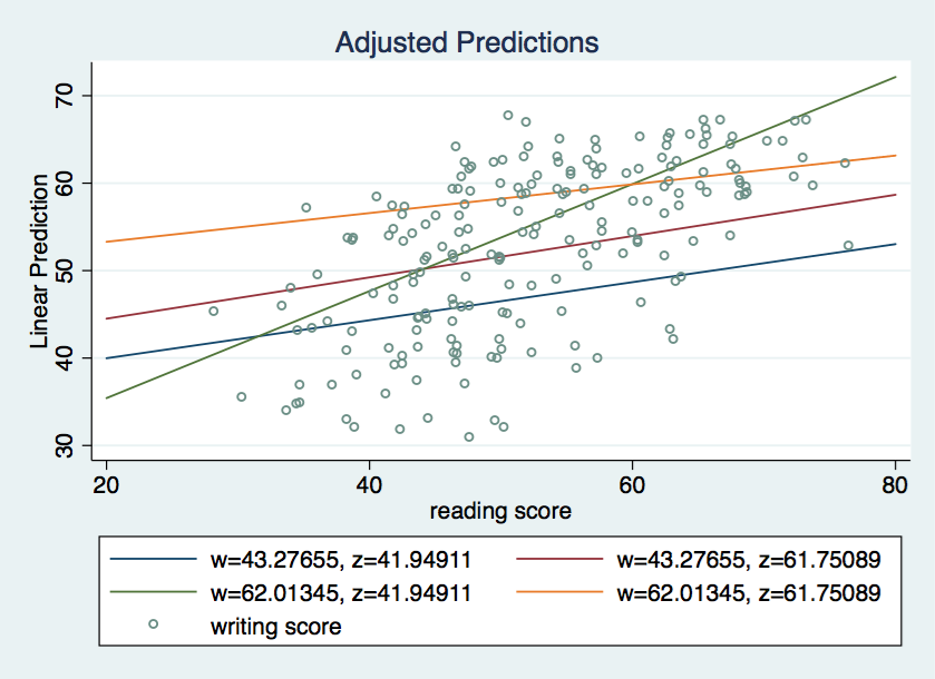
Now we have a good idea of what is going on with these data.
Hey, wait a minute, my model also has covariates. What about them?
We will deal with adding covariates to the model in
the next section.
Three-way interaction of continuous variables with covariates
Here is the regression model from the previous page with two covariates V1 and V2 added.
Y = b0 + b1X + b2Z + b3W + b4XZ + b5XW + b6ZW + b7XZW + b8V1 + b9V2
Adding covariates to your model does not change the formulas for the simple
slopes as long as the covariates are not interacted with the independent variable or the
moderator variables.
We will add two covariates to our previous model, socst which will be renamed as v1 and
ses which will be renamed v2. Everything is this section is the
same as the previous example with the exception of adding the covariates to the end
of the regress command.
rename socst v1
rename ses v2

regress y c.x##c.z##c.w v1 v2

      Source |       SS       df       MS              Number of obs =     200
-------------+------------------------------           F(  9,   190) =   25.36
       Model |  9757.27668     9  1084.14185           Prob > F      =  0.0000
    Residual |  8121.59832   190  42.7452543           R-squared     =  0.5457
-------------+------------------------------           Adj R-squared =  0.5242
       Total |   17878.875   199   89.843593           Root MSE      =   6.538

------------------------------------------------------------------------------
           y |      Coef.   Std. Err.      t    P>|t|     [95% Conf. Interval]
-------------+----------------------------------------------------------------
           x |  -3.463037   1.716525    -2.02   0.045    -6.848932   -.0771426
           z |  -2.902201   1.670106    -1.74   0.084    -6.196533    .3921302
             |
     c.x#c.z |   .0624411     .03093     2.02   0.045     .0014308    .1234514
             |
           w |  -3.696588   1.831366    -2.02   0.045    -7.309009   -.0841671
             |
     c.x#c.w |   .0796921   .0341529     2.33   0.021     .0123245    .1470597
             |
     c.z#c.w |   .0696334   .0332851     2.09   0.038     .0039775    .1352893
             |
 c.x#c.z#c.w |  -.0013838   .0005968    -2.32   0.021    -.0025611   -.0002065
             |
          v1 |   .2789791    .057697     4.84   0.000     .1651703     .392788
          v2 |  -.9056562   .6914623    -1.31   0.192    -2.269585    .4582727
       _cons |   185.3134   88.56438     2.09   0.038      10.6177    360.0092
------------------------------------------------------------------------------
Note that with the inclusion the covariates that the three-way
interaction is even “more” significant than before.
Next, we will compute the simple slopes for the various combinations of w
and z. The margins command is exactly the same as for the example without
the covariates because the covariances are not involved in the 3-way interaction.
/* compute simple slopes */

margins, dydx(x) at(w=($Hw $Lw) z=($Hz $Lz)) vsquish

Average marginal effects                          Number of obs   =        200
Model VCE    : OLS

Expression   : Linear prediction, predict()
dy/dx w.r.t. : x
1._at        : z               =    61.75089
               w               =    62.01345
2._at        : z               =    61.75089
               w               =    43.27655
3._at        : z               =    41.94911
               w               =    62.01345
4._at        : z               =    41.94911
               w               =    43.27655

------------------------------------------------------------------------------
             |            Delta-method
             |      dy/dx   Std. Err.      z    P>|z|     [95% Conf. Interval]
-------------+----------------------------------------------------------------
x            |
         _at |
          1  |   .0356648   .0951734     0.37   0.708    -.1508717    .2222012
          2  |   .1435565   .1371306     1.05   0.295    -.1252146    .4123276
          3  |    .498484   .1884961     2.64   0.008     .1290384    .8679296
          4  |   .0929561   .1236172     0.75   0.452    -.1493291    .3352413
------------------------------------------------------------------------------
Let’s plot the four simple slopes on top of the observations.
We begin the graphing by computing expected values using the margins
command for different values of ww and z.
Again, we need only
two values of x (20 & 80) to define each simple slope regression line.
margins, at(x=(20 80) w=($Hw $Lw) z=($Hz $Lz)) vsquish

Predictive margins                                Number of obs   =        200
Model VCE    : OLS

Expression   : Linear prediction, predict()
1._at        : x               =          20
               z               =    61.75089
               w               =    62.01345
2._at        : x               =          20
               z               =    61.75089
               w               =    43.27655
3._at        : x               =          20
               z               =    41.94911
               w               =    62.01345
4._at        : x               =          20
               z               =    41.94911
               w               =    43.27655
5._at        : x               =          80
               z               =    61.75089
               w               =    62.01345
6._at        : x               =          80
               z               =    61.75089
               w               =    43.27655
7._at        : x               =          80
               z               =    41.94911
               w               =    62.01345
8._at        : x               =          80
               z               =    41.94911
               w               =    43.27655

------------------------------------------------------------------------------
             |            Delta-method
             |     Margin   Std. Err.      z    P>|z|     [95% Conf. Interval]
-------------+----------------------------------------------------------------
         _at |
          1  |   56.98694   3.936984    14.47   0.000     49.27059    64.70329
          2  |   47.84013   4.825798     9.91   0.000     38.38174    57.29852
          3  |   38.20389   6.500797     5.88   0.000     25.46256    50.94522
          4  |   44.62434   3.040215    14.68   0.000     38.66563    50.58306
          5  |   59.12683   2.060024    28.70   0.000     55.08925     63.1644
          6  |   56.45352   3.835255    14.72   0.000     48.93656    63.97048
          7  |   68.11293   5.302337    12.85   0.000     57.72054    78.50532
          8  |   50.20171   4.580553    10.96   0.000     41.22399    59.17943
------------------------------------------------------------------------------

marginsplot, recast(line) noci addplot(scatter y x, msym(oh) jitter(3))
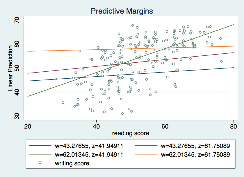
With the covariates in the model we have a bit more variation in the simple slopes. However,
once again it looks like slope 3 is the one that is the most different from the others.
We can compute tests of differences in simple slopes using the pwcompare(effects) option
for margins. This option was introduced in Stata 12.
/* compute pairwise differences in simple slopes */

margins, dydx(x) at(w=($Hw $Lw) z=($Hz $Lz)) vsquish pwcompare(effects)

Pairwise comparisons of average marginal effects
Model VCE    : OLS

Expression   : Linear prediction, predict()
dy/dx w.r.t. : x
1._at        : z               =    61.75089
               w               =    62.01345
2._at        : z               =    61.75089
               w               =    43.27655
3._at        : z               =    41.94911
               w               =    62.01345
4._at        : z               =    41.94911
               w               =    43.27655

------------------------------------------------------------------------------
             |   Contrast Delta-method    Unadjusted           Unadjusted
             |      dy/dx   Std. Err.      z    P>|z|     [95% Conf. Interval]
-------------+----------------------------------------------------------------
x            |
         _at |
     2 vs 1  |   .1078917   .1559956     0.69   0.489     -.197854    .4136375
     3 vs 1  |   .4628192   .1955057     2.37   0.018     .0796352    .8460033
     4 vs 1  |   .0572913   .1557822     0.37   0.713    -.2480361    .3626188
     3 vs 2  |   .3549275   .2449055     1.45   0.147    -.1250785    .8349335
     4 vs 2  |  -.0506004   .1635762    -0.31   0.757    -.3712038    .2700031
     4 vs 3  |  -.4055279   .2096843    -1.93   0.053    -.8165015    .0054457
------------------------------------------------------------------------------
Inspecting the table above it appears slope 3 versus slope 1 (LzHw vs HzHw) is the only
one of the tests that is significant. But before we reach that conclusion we will need
to adjust the p-values to take into account that these are post-hoc tests. To do this,
we will add the mcompare(bonferroni) option to the margins command.
/* compute pairwise differences in simple slopes with Bonferroni correction */

margins, dydx(x) at(w=($Hw $Lw) z=($Hz $Lz)) vsquish pwcompare(effects) mcompare(bonferroni)

Pairwise comparisons of average marginal effects
Model VCE    : OLS

Expression   : Linear prediction, predict()
dy/dx w.r.t. : x
1._at        : z               =    61.75089
               w               =    62.01345
2._at        : z               =    61.75089
               w               =    43.27655
3._at        : z               =    41.94911
               w               =    62.01345
4._at        : z               =    41.94911
               w               =    43.27655

---------------------------
             |    Number of
             |  Comparisons
-------------+-------------
x            |
         _at |            6
---------------------------

------------------------------------------------------------------------------
             |   Contrast Delta-method    Bonferroni           Bonferroni
             |      dy/dx   Std. Err.      z    P>|z|     [95% Conf. Interval]
-------------+----------------------------------------------------------------
x            |
         _at |
     2 vs 1  |   .1078917   .1559956     0.69   1.000    -.3036648    .5194483
     3 vs 1  |   .4628192   .1955057     2.37   0.108     -.052975    .9786135
     4 vs 1  |   .0572913   .1557822     0.37   1.000    -.3537022    .4682849
     3 vs 2  |   .3549275   .2449055     1.45   0.884    -.2911963    1.001051
     4 vs 2  |  -.0506004   .1635762    -0.31   1.000    -.4821564    .3809557
     4 vs 3  |  -.4055279   .2096843    -1.93   0.319    -.9587289    .1476731
------------------------------------------------------------------------------
With the Bonferroni correction the p-value for 3 vs 1 becomes 0.108,
which is not statistically significant.
The Bonferroni correction may not be the best choice because it is overly conservative but it
is certainly easy to implement.
References
Dawson, J.F. & Richter, A.W. (2004) A significance test of slope differences for
three-way interactions in moderated multiple regression analysis. RP0422.
Aston University, Birmingham, UK