
Stata has several procedures that can be used in analyzing count data. Let’s begin by loading
and describing a dataset on 316 students at two Los Angeles high schools.
use https://stats.idre.ucla.edu/stat/stata/notes/lahigh, clear

describe

Contains data from lahigh.dta
  obs:           316
 vars:            10                          3 Dec 1999 09:43
 size:        13,904 (98.5% of memory free)   (_dta has notes)
-------------------------------------------------------------------------------
   1. id        float  %9.0g
   2. gender    float  %9.0g       gl
   3. ethnic    float  %10.0g      el         ethnicity
   4. school    float  %9.0g                  school 1 or 2
   5. mathpr    float  %9.0g                  ctbs math pct rank
   6. langpr    float  %9.0g                  ctbs lang pct rank
   7. mathnce   float  %9.0g                  ctbs math nce
   8. langnce   float  %9.0g                  ctbs lang nce
   9. biling    float  %12.0g      bl         bilingual status
  10. daysabs   float  %9.0g                  number days absent
-------------------------------------------------------------------------------
Sorted by:
Let’s analyze the variable daysabs to see if there is an effect due to gender and ability as measured by
mathnce and langnce. To begin with, we have always been warned against
using count data in OLS regression. A simple histogram can show us that this is a good recommendation.
hist daysabs
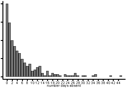
The data are strongly skewed to the right, so clearly OLS regression would be
inappropriate. Count data often follow a poisson distribution, so some type of poisson
analysis might be appropriate. Recall from statistical theory that in a poisson distribution the
mean and variance are the same. Let’s summarize daysabs using the detail option.
summarize daysabs, detail

                     number days absent
-------------------------------------------------------------
      Percentiles      Smallest
 1%            0              0
 5%            0              0
10%            0              0       Obs                 316
25%            1              0       Sum of Wgt.         316

50%            3                      Mean           5.810127
                        Largest       Std. Dev.      7.449003
75%            8             35
90%           14             35       Variance       55.48764
95%           23             41       Skewness       2.250587
99%           35             45       Kurtosis       8.949302
The variance of daysabs is nearly 10 times larger than the mean. The distribution
of daysabs is displaying signs of overdispersion, that is, greater variance than
might be expected in a poisson distribution. Before we get to an alternative analysis,
let’s run a poisson regression, even though we believe that the poisson distribution is not correct.
Poisson regression can be followed up with the poisgof command which tests the poisson
goodness-of-fit. Here is what these commands look like.
poisson daysabs gender mathnce langnce

Iteration 0:   log likelihood = -1547.9709
Iteration 1:   log likelihood = -1547.9709

Poisson regression                                Number of obs   =        316
                                                  LR chi2(3)      =     175.27
                                                  Prob > chi2     =     0.0000
Log likelihood = -1547.9709                       Pseudo R2       =     0.0536

------------------------------------------------------------------------------
 daysabs |      Coef.   Std. Err.       z     P>|z|       [95% Conf. Interval]
---------+--------------------------------------------------------------------
  gender |  -.4009209   .0484122     -8.281   0.000       -.495807   -.3060348
 mathnce |  -.0035232   .0018213     -1.934   0.053       -.007093    .0000466
 langnce |  -.0121521   .0018348     -6.623   0.000      -.0157483   -.0085559
   _cons |   3.088587   .1017365     30.359   0.000       2.889187    3.287987
------------------------------------------------------------------------------

* Stata 8 code.
poisgof

* Stata 9 and 10 code and output.
estat gof

Goodness of fit chi-2 =  2234.546
Prob > chi2(312)      =    0.0000
The large value for chi-square in the gof is another indicator that the poisson
distribution is not a good choice. A significant (p<0.05) test statistic from the gof
indicates that the poisson model is inapproprite. Let’s run the analysis one more time, this time using negative binomial regression. Negative binomial regression is often more appropriate in cases of overdispersion. Here
is the negative binomial analysis.
nbreg daysabs gender mathnce langnce

Fitting comparison Poisson model:

Iteration 0:   log likelihood = -1547.9709
Iteration 1:   log likelihood = -1547.9709

Fitting constant-only model:

Iteration 0:   log likelihood = -897.78991
Iteration 1:   log likelihood = -891.24455
Iteration 2:   log likelihood = -891.24271
Iteration 3:   log likelihood = -891.24271

Fitting full model:

Iteration 0:   log likelihood = -881.57337
Iteration 1:   log likelihood = -880.87788
Iteration 2:   log likelihood = -880.87312
Iteration 3:   log likelihood = -880.87312

Negative binomial regression                      Number of obs   =        316
                                                  LR chi2(3)      =      20.74
                                                  Prob > chi2     =     0.0001
Log likelihood = -880.87312                       Pseudo R2       =     0.0116

------------------------------------------------------------------------------
 daysabs |      Coef.   Std. Err.       z     P>|z|       [95% Conf. Interval]
---------+--------------------------------------------------------------------
  gender |  -.4311844   .1396656     -3.087   0.002       -.704924   -.1574448
 mathnce |   -.001601     .00485     -0.330   0.741      -.0111067    .0079048
 langnce |  -.0143475   .0055815     -2.571   0.010      -.0252871    -.003408
   _cons |   3.147254   .3211669      9.799   0.000       2.517778    3.776729
---------+--------------------------------------------------------------------
/lnalpha |   .2533877   .0955362                          .0661402    .4406351
---------+--------------------------------------------------------------------
   alpha |   1.288383   .1230871     10.467   0.000       1.068377    1.553694
------------------------------------------------------------------------------
Likelihood ratio test of alpha=0:    chi2(1) =  1334.20   Prob > chi2 = 0.0000
The likelihood ratio test at the bottom of the analysis is a test of the overdispersion
parameter alpha. When the overdispersion parameter is zero the negative binomial distrbution is
equivalent to a poisson distribution. In this case, alpha is significantly different from zero
and thus reinforces one last time that the poisson distribution is not appropriate.
In the analysis itself, both gender and langnce are significant while
mathnce
is not. From the coding of gender (1=female, 2=male) it is evident that females are absent
significantly more than are males. The significant coefficient for langnce suggests that
higher ability students are absent less often than lower ability students.