
When modeling a count variable, there are several available models to choose
from. Stata supports Poisson, negative binomial, zero-inflated Poisson,
zero-inflated negative binomial models, zero-truncated Poisson, and
zero-truncated negative binomial models. Among these, you can likely
narrow your data down to one or two models based on how the data were collected
and the distribution of your outcome variable.
Some important questions to ask yourself before you start building a count model
are:
- Does my outcome variable contain zeroes?
- If yes, what does a zero mean?
- If no, why not?
- How is my outcome variable distributed?
- What is the variance of my outcome variable?
- How does the variance compare to the mean?
The answers to the first set of questions can indicate whether your data are
zero-truncated or zero-inflated.
If your count variable does not contain zeroes…
ask yourself why. Given what you know about the variable, would you have
expected to see counts of zero? In some instances, a count of zero will
never appear in the dataset. For example, if your count variable is the number
of visits to a given coffee shop in a week and your data are collected among people
in the coffee shop,
then all the people for whom you collected data have a count of at least one. A
person who never visits the coffee shop will not be included in the dataset. This
is an example of zero-truncated data and would most appropriately be
modeled using a zero-truncated model. However, just because a variable
does not contain zeroes does not mean the variable is zero-truncated.
Truncation occurs because of the way in which the data are collected and cannot
be assumed just from looking at the data.
If your count variable does contain zeroes…
again,
ask yourself why.
What does a count of zero mean, given what you know about the variable? In some
instances, records in a dataset could ONLY have counts of zero. For
examples, if you are collecting data on the number of fish caught by a person in
a given weekend, a person who did not go fishing could only have a count of
zero. A person who did go fishing could also have a count of zero, but these two
zeroes would have very different meanings. This is an example of
zero-inflated data and may be most appropriately modeled with a
zero-inflated model.
The answers to the second set of questions can indicate whether a Poisson or negative
binomial distribution is more appropriate for your data. The Poisson
distribution is characterized by equal mean and variance. If the sample mean and
sample variance of your outcome variable are in the same neighborhood, a Poisson
model may be appropriate. If the variance exceeds the mean by a great deal, a
negative binomial model may be appropriate. Keep in mind that zero-truncation
and zero-inflation can impact these statistics and there is not a magical
cut-off determining when one model is better than the other. These are simply
aspects of your data worth considering.
Deciding on a final model
You may find that, after making all of the above considerations and deciding
which predictors should be included in your model, you are still torn. You have
two count models that both seem substantively reasonable, but that are clearly
mathematically different. At this point, the countfit function in Stata
(written by Long and Freese) can be a helpful tool. You can download it by
typing search countfit (see How can I
use the search command to search for programs and get additional help? for
more information about using search) and following the appropriate links.
Countfit runs user-specified count models (Poisson, zero-inflated
Poisson, negative binomial, and zero-inflated negative binomial) with
user-specified variables and compares the model residuals. If you do not
indicate which models you wish to compare (nbreg, zinp, prm,
or zip), countfit will default to
running and comparing all four. One if the quirks of countfit is that it displays results for a given predictor next to the predictor’s
label rather than name. So
an unlabeled predictor will lead to both empty space in the output and possible
confusion. This can be prevented by labeling ALL predictors before running
countfit.
In this example, we will be looking at academic information on
316 students. The response variable is days absent during the school year (daysabs).
We have narrowed our model choices down to two negative binomial models, one
with zero-inflation and one without. We believe that the daysabs can best
be predicted with math standardized tests score (mathnce),
language standardized tests score (langnce) and gender (female).
We suspect certain zeroes can be predicted with bilingual status (biling)
and language score (langnce). We will run the countfit command
indicating these predictors and the two models we wish to compare,
then discuss the output.
use https://stats.idre.ucla.edu/stat/stata/notes/lahigh, clear

generate female = (gender == 1)
label variable female `"female"'countfit daysabs mathnce langnce female, inf(biling langnce) nbreg zinb
----------------------------------------------------------
                        Variable |   NBRM        ZINB
---------------------------------+------------------------
daysabs                          |
                   ctbs math nce |     0.998       0.998
                                 |     -0.33       -0.34
                   ctbs lang nce |     0.986       0.987
                                 |     -2.57       -2.38
                          female |     1.539       1.502
                                 |      3.09        2.94
                        Constant |     9.825       9.795
                                 |     10.89       10.94
---------------------------------+------------------------
lnalpha                          |
                        Constant |     1.288       1.191
                                 |      2.65        1.62
---------------------------------+------------------------
inflate                          |
                bilingual status |                10.132
                                 |                  1.53
                   ctbs lang nce |                 1.094
                                 |                  1.92
                        Constant |                 0.000
                                 |                 -2.16
---------------------------------+------------------------
Statistics                       |
                           alpha |     1.288
                               N |   316.000     316.000
                              ll |  -880.873    -879.131
                             bic |  1790.525    1804.307
                             aic |  1771.746    1774.262
----------------------------------------------------------
                                               legend: b/t
Comparison of Mean Observed and Predicted Count

            Maximum       At      Mean
Model     Difference    Value    |Diff|
---------------------------------------------
NBRM        0.011         1      0.004
ZINB        0.018         1      0.005

NBRM: Predicted and actual probabilities

Count   Actual    Predicted    |Diff|   Pearson
------------------------------------------------
0        0.196       0.201      0.004     0.031
1        0.146       0.135      0.011     0.278
2        0.098       0.104      0.006     0.093
3        0.082       0.083      0.001     0.004
4        0.070       0.068      0.001     0.008
5        0.063       0.057      0.006     0.230
6        0.047       0.048      0.000     0.001
7        0.038       0.040      0.002     0.046
8        0.028       0.034      0.006     0.318
9        0.035       0.029      0.005     0.319
------------------------------------------------
Sum      0.804       0.799      0.044     1.327

ZINB: Predicted and actual probabilities

Count   Actual    Predicted    |Diff|   Pearson
------------------------------------------------
0        0.196       0.207      0.011     0.176
1        0.146       0.127      0.018     0.850
2        0.098       0.101      0.003     0.022
3        0.082       0.082      0.000     0.000
4        0.070       0.068      0.001     0.007
5        0.063       0.057      0.006     0.194
6        0.047       0.048      0.001     0.006
7        0.038       0.041      0.003     0.077
8        0.028       0.035      0.007     0.393
9        0.035       0.030      0.005     0.240
------------------------------------------------
Sum      0.804       0.798      0.055     1.965

Tests and Fit Statistics

-------------------------------------------------------------------------
NBRM           BIC=   -28.290  AIC=     5.607  Prefer  Over  Evidence
-------------------------------------------------------------------------
  vs ZINB      BIC=   -14.507  dif=   -13.783  NBRM    ZINB  Very strong
               AIC=     5.615  dif=    -0.008  NBRM    ZINB
               Vuong=   0.858  prob=    0.195  ZINB    NBRM  p=0.195
Making sense of the output
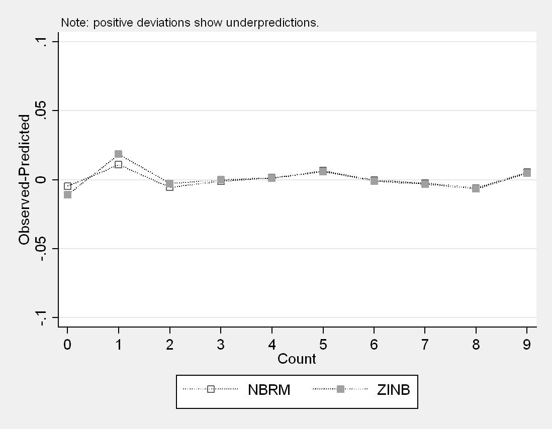
First, let’s discuss the graph. Countfit produces a graph that plots the residuals from the tested models. Small residuals are indicative of good-fitting
models, so the models with lines closest to zero should be considered for our
data. This may be useful in eliminating a model, but be careful
about deciding on one model over all the others based solely on this graph.
In the graph above, we see that our two models perform very similarly for counts
greater than two, and that they both differ most from the actual values and each other at the
zero and one counts. At the zero and one counts, the negative binomial
model appears slightly better than the zero-inflated negative binomial model.
Model parameters and fit
The first table in the output summarizes the parameter estimates from each of
the tested models. For each of the models, we see the exponentiated
coefficients and their t-statistics in the first block of the table.
Then, for any negative binomial models, we will see the estimated dispersion parameters.
Next, for any zero-inflated models, we see the estimates from the logistic model
predicting the certain zeroes. In the last block of the table, a set of fit
statistics is provided for each of the four models. This includes the
log-likelihood, BIC, and AIC.
----------------------------------------------------------
                        Variable |   NBRM        ZINB
---------------------------------+------------------------
daysabs                          |
                   ctbs math nce |     0.998       0.998
                                 |     -0.33       -0.34
                   ctbs lang nce |     0.986       0.987
                                 |     -2.57       -2.38
                          female |     1.539       1.502
                                 |      3.09        2.94
                        Constant |     9.825       9.795
                                 |     10.89       10.94
---------------------------------+------------------------
lnalpha                          |
                        Constant |     1.288       1.191
                                 |      2.65        1.62
---------------------------------+------------------------
inflate                          |
                bilingual status |                10.132
                                 |                  1.53
                   ctbs lang nce |                 1.094
                                 |                  1.92
                        Constant |                 0.000
                                 |                 -2.16
---------------------------------+------------------------
Statistics                       |
                           alpha |     1.288
                               N |   316.000     316.000
                              ll |  -880.873    -879.131
                             bic |  1790.525    1804.307
                             aic |  1771.746    1774.262
----------------------------------------------------------
                                               legend: b/t
From the last block, we can see that the two models are extremely
close. The parameter estimates are nearly identical. We can continue to look at
the rest of the output.
Residuals by count
Next, we see a table with one line per model showing the maximum and mean
differences in observed versus predicted counts.
Comparison of Mean Observed and Predicted Count

            Maximum       At      Mean
Model     Difference    Value    |Diff|
---------------------------------------------
NBRM        0.011         1      0.004
ZINB        0.018         1      0.005
This confirms what we observed in the graph: both models performed worst when
predicting a count of 1. Between these two, we see that the negative binomial
did better at this prediction and, overall, had a lower mean absolute difference
between predicted and observed values. At this point, the negative binomial
model is looking more appropriate than the zero-inflated negative binomial
model. Next, we have one table for each of the models containing count-by-count
information.
NBRM: Predicted and actual probabilities

Count   Actual    Predicted    |Diff|   Pearson
------------------------------------------------
0        0.196       0.201      0.004     0.031
1        0.146       0.135      0.011     0.278
2        0.098       0.104      0.006     0.093
3        0.082       0.083      0.001     0.004
4        0.070       0.068      0.001     0.008
5        0.063       0.057      0.006     0.230
6        0.047       0.048      0.000     0.001
7        0.038       0.040      0.002     0.046
8        0.028       0.034      0.006     0.318
9        0.035       0.029      0.005     0.319
------------------------------------------------
Sum      0.804       0.799      0.044     1.327

ZINB: Predicted and actual probabilities

Count   Actual    Predicted    |Diff|   Pearson
------------------------------------------------
0        0.196       0.207      0.011     0.176
1        0.146       0.127      0.018     0.850
2        0.098       0.101      0.003     0.022
3        0.082       0.082      0.000     0.000
4        0.070       0.068      0.001     0.007
5        0.063       0.057      0.006     0.194
6        0.047       0.048      0.001     0.006
7        0.038       0.041      0.003     0.077
8        0.028       0.035      0.007     0.393
9        0.035       0.030      0.005     0.240
------------------------------------------------
Sum      0.804       0.798      0.055     1.965
In these two tables, we are able to see, for counts 0-9, the actual
proportion of our data records with the given count and the predicted proportion
from each models. The absolute
difference is included, as is the given count’s contribution to a Pearson
Chi-Square statistic comparing the actual distribution of the data and the
distribution proposed by the model. For a given row, the Pearson statistic can
be calculated as N(|Diff|2)/Predicted, where N is the number of
observations in the dataset. Looking at the sum of the Pearson column
gives us a sense of how close the predicted proportions were to the actual
proportions. Using this method to compare, the negative binomial appears better
than the zero-inflated negative binomial.
Summary comparisons
Tests and Fit Statistics

-------------------------------------------------------------------------
NBRM           BIC=   -28.290  AIC=     5.607  Prefer  Over  Evidence
-------------------------------------------------------------------------
  vs ZINB      BIC=   -14.507  dif=   -13.783  NBRM    ZINB  Very strong
               AIC=     5.615  dif=    -0.008  NBRM    ZINB
               Vuong=   0.858  prob=    0.195  ZINB    NBRM  p=0.195
In this table, the tested models are compared to each other head-to-head using
the tests appropriate to each comparison. Each line can be boiled down to
the last three columns. They suggest which model is preferred by the given
comparison and the strength of the evidence supporting this preference.
When we compare our two models using the BIC and AIC,
the negative binomial is preferred over zero-inflated negative
binomial. The Vuong test prefers zero-inflated negative binomial model over the
negative binomial model, but not at a statistically significant level.
Thus, these model fit statistics support what we have seen in the model
residuals.
Full model output
There may be times when you wish to see the full model output for each of the
four models. This can be especially helpful in choosing between two models
because it allows you to see the significance levels of the parameters, which
are not included in the countfit output. For instance, in this
example, we might be interested in the significance levels of our zero-inflated
variables. To do
this, you can add the noisily option to the countfit command:
countfit daysabs mathnce langnce female, inf(biling langnce) nbreg zinb noisily
This will print the full output from each of the four models, then the summary output provided without the
noisily option.
Replace option
When you run countfit, variables are generated
and added to your dataset. If you ran the same countfit command a
second time, you would encounter error messages telling you that variables have
already been defined. Thus, if you are running multiple countfit tests,
you can add the replace option to your command to replace the variables
generated by prior runs with the variables generated by the current run.
Final thoughts
Countfit presents
several nice ways for you to compare models that are not necessarily easy to
compare. It presents side-by-side fit statistics and parameter estimates, it
gives you a graphical representation of the model residuals, as well as a table
of the residuals by counts. All of these pieces of information are worth taking
into consideration when choosing a model. For your purposes, some of these
measures may be more relevant than the others. Think carefully about what you
are aiming to do in the model and which measures should be prioritized over
others. While countfit is very convenient and provides lots of
information, sorting through the information it provides must be done carefully.