
This page is just an extension of How can I do moderated mediation
in Stata? to include a categorical moderator variables.
We will call that page modmed. If
you are unfamiliar with moderated mediation you should review the modmed
FAQ page before continuing on with this page.
We will to use the same data and the same abbreviated variable names as were used on the
modmed page. The model is not of substantive interest, it is merely
used to show the steps involved in the analysis.
use https://stats.idre.ucla.edu/stat/data/hsbdemo, clear
rename science y  /* dependent variable   */
rename math x     /* independent variable */
rename read m     /* mediator variable    */
rename female w   /* moderator variable with 2 levels */
rename socst cv   /* continuous covariate */
The modmed page presented five different models for moderated mediation.
This page will cover models 5, 2 and 3, to illustrate the use of categorical moderators.
The diagram for model 5 looks like this:
Model 5
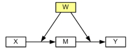
First pass using sem
The trick to using sem for moderated mediation with a categorical moderator
is to do a multiple group
analysis using the group option. Please note, there are no explicit
interactions in the model. The interactions are implicit in the multiple group analysis
itself. Here is our first try.
sem (m <- x cv)(y <- m x cv), group(w)

Endogenous variables

Observed:  m y

Exogenous variables

Observed:  x cv

Fitting target model:

Iteration 0:   log likelihood = -2792.7769
Iteration 1:   log likelihood = -2792.7769

Structural equation model                       Number of obs      =       200
Grouping variable  = w                          Number of groups   =         2
Estimation method  = ml
Log likelihood     = -2792.7769

------------------------------------------------------------------------------
             |                 OIM
             |      Coef.   Std. Err.      z    P>|z|     [95% Conf. Interval]
-------------+----------------------------------------------------------------
Structural   |
  m <-       |
    x        |
        male |   .4461113     .09393     4.75   0.000      .262012    .6302107
      female |   .5523602   .0843711     6.55   0.000     .3869959    .7177244
    cv       |
        male |   .3687237   .0800976     4.60   0.000     .2117353     .525712
      female |   .3444715   .0754397     4.57   0.000     .1966124    .4923306
    _cons    |
        male |   10.10814    4.69041     2.16   0.031     .9151099    19.30118
      female |   4.564765   3.855135     1.18   0.236    -2.991162    12.12069
  -----------+----------------------------------------------------------------
  y <-       |
    m        |
        male |   .4504614   .1045896     4.31   0.000     .2454696    .6554532
      female |    .211106   .0977165     2.16   0.031     .0195853    .4026267
    x        |
        male |   .3523138   .1046885     3.37   0.001     .1471281    .5574996
      female |    .452633   .1015976     4.46   0.000     .2535052    .6517607
    cv       |
        male |   .0497414   .0887335     0.56   0.575    -.1241731     .223656
      female |   .0458989   .0840018     0.55   0.585    -.1187416    .2105395
    _cons    |
        male |   8.206073   4.797652     1.71   0.087    -1.197152     17.6093
      female |   13.63157   3.958183     3.44   0.001     5.873677    21.38947
-------------+----------------------------------------------------------------
Variance     |
  e.m        |
        male |   55.76584   8.267278                        41.704    74.56907
      female |   41.59327   5.634104                      31.89494    54.24058
  e.y        |
        male |   55.51193   8.229635                      41.51411    74.22955
      female |   43.28974   5.863902                      33.19584     56.4529
------------------------------------------------------------------------------
LR test of model vs. saturated: chi2(0)   =      0.00, Prob > chi2 =      .
This isn’t too bad. We are getting separate male and female coefficients for both
x and m. However, we are also getting separate
coefficients for cv and separate residual variances in each equations.
In a traditional moderated mediation model these values are not part of the interaction.
So, we will need to constrain the coefficients for cv and residual variances to
be equal in both equations. Here is how to do that.
Model 5 constraining the covariate to be equal across groups
Equations that begin with 0: refer to the male group and equations that begin with 1: refer
to the female group. To constrain values use a ‘@’ and a name. Terms with the same name
will be constrained to be equal. For example, the term cv@c1 will be
constrained to be equal in both equations.
sem (0: m <- x cv@c1)(0: y <- m x cv@c2) ///
    (1: m <- x cv@c1)(1: y <- m x cv@c2), group(w) ///
    variance(0: e.m@v1 e.y@v2) ///
    variance(1: e.m@v1 e.y@v2)

Endogenous variables

Observed:  m y

Exogenous variables

Observed:  x cv

Fitting target model:

Iteration 0:   log likelihood = -2795.5195
Iteration 1:   log likelihood = -2794.6484
Iteration 2:   log likelihood = -2794.6438
Iteration 3:   log likelihood = -2794.6438

Structural equation model                       Number of obs      =       200
Grouping variable  = w                          Number of groups   =         2
Estimation method  = ml
Log likelihood     = -2794.6438

 ( 1)  [m]0bn.w#c.cv - [m]1.w#c.cv = 0
 ( 2)  [y]0bn.w#c.cv - [y]1.w#c.cv = 0
 ( 3)  [var(e.m)]0bn.w - [var(e.m)]1.w = 0
 ( 4)  [var(e.y)]0bn.w - [var(e.y)]1.w = 0
------------------------------------------------------------------------------
             |                 OIM
             |      Coef.   Std. Err.      z    P>|z|     [95% Conf. Interval]
-------------+----------------------------------------------------------------
Structural   |
  m <-       |
    x        |
        male |   .4525824   .0821032     5.51   0.000      .291663    .6135017
      female |   .5435942   .0815035     6.67   0.000     .3838503    .7033381
    cv       |
         [*] |   .3576463   .0548017     6.53   0.000     .2502369    .4650556
    _cons    |
        male |   10.33924   4.225914     2.45   0.014     2.056605    18.62188
      female |   4.326879   4.000737     1.08   0.279    -3.514422    12.16818
  -----------+----------------------------------------------------------------
  y <-       |
    m        |
        male |   .4513773   .0937037     4.82   0.000     .2677214    .6350331
      female |   .2101483   .0992473     2.12   0.034     .0156271    .4046694
    x        |
        male |   .3527524   .0972145     3.63   0.000     .1622155    .5432893
      female |   .4520144   .1061237     4.26   0.000     .2440157    .6600131
    cv       |
         [*] |   .0479536   .0608685     0.79   0.431    -.0713466    .1672537
    _cons    |
        male |   8.227069   4.450954     1.85   0.065    -.4966419    16.95078
      female |    13.6048   4.117905     3.30   0.001     5.533856    21.67575
-------------+----------------------------------------------------------------
Variance     |
  e.m        |
         [*] |   48.05346   4.805346                      39.50068    58.45812
  e.y        |
         [*] |   48.85108   4.885108                      40.15633    59.42843
------------------------------------------------------------------------------
Note: [*] identifies parameter estimates constrained to be equal across
      groups.
LR test of model vs. saturated: chi2(4)   =      3.73, Prob > chi2 = 0.4432
Now we can use the estat teffects to calculate the indirect
effects for both males and females.
estat teffects


Direct effects
------------------------------------------------------------------------------
             |                 OIM
             |      Coef.   Std. Err.      z    P>|z|     [95% Conf. Interval]
-------------+----------------------------------------------------------------
Structural   |
  m <-       |
    x        |
        male |   .4525824   .0821032     5.51   0.000      .291663    .6135017
      female |   .5435942   .0815035     6.67   0.000     .3838503    .7033381
    cv       |
        male |   .3576463   .0548017     6.53   0.000     .2502369    .4650556
      female |   .3576463   .0548017     6.53   0.000     .2502369    .4650556
  -----------+----------------------------------------------------------------
  y <-       |
    m        |
        male |   .4513773   .0937037     4.82   0.000     .2677214    .6350331
      female |   .2101483   .0992473     2.12   0.034     .0156271    .4046694
    x        |
        male |   .3527524   .0972145     3.63   0.000     .1622155    .5432893
      female |   .4520144   .1061237     4.26   0.000     .2440157    .6600131
    cv       |
        male |   .0479536   .0608685     0.79   0.431    -.0713466    .1672537
      female |   .0479536   .0608685     0.79   0.431    -.0713466    .1672537
------------------------------------------------------------------------------


Indirect effects
------------------------------------------------------------------------------
             |                 OIM
             |      Coef.   Std. Err.      z    P>|z|     [95% Conf. Interval]
-------------+----------------------------------------------------------------
Structural   |
  m <-       |
    x        |
         [*] |          0  (no path)
    cv       |
         [*] |          0  (no path)
  -----------+----------------------------------------------------------------
  y <-       |
    m        |
         [*] |          0  (no path)
    x        |
        male |   .2042854   .0563196     3.63   0.000     .0939009    .3146699
      female |   .1142354   .0566038     2.02   0.044     .0032939    .2251768
    cv       |
        male |   .1614334   .0416532     3.88   0.000     .0797947    .2430722
      female |   .0751587    .037317     2.01   0.044     .0020188    .1482986
------------------------------------------------------------------------------
Note: [*] identifies parameter estimates constrained to be equal across
      groups.


Total effects
------------------------------------------------------------------------------
             |                 OIM
             |      Coef.   Std. Err.      z    P>|z|     [95% Conf. Interval]
-------------+----------------------------------------------------------------
Structural   |
  m <-       |
    x        |
        male |   .4525824   .0821032     5.51   0.000      .291663    .6135017
      female |   .5435942   .0815035     6.67   0.000     .3838503    .7033381
    cv       |
        male |   .3576463   .0548017     6.53   0.000     .2502369    .4650556
      female |   .3576463   .0548017     6.53   0.000     .2502369    .4650556
  -----------+----------------------------------------------------------------
  y <-       |
    m        |
        male |   .4513773   .0937037     4.82   0.000     .2677214    .6350331
      female |   .2101483   .0992473     2.12   0.034     .0156271    .4046694
    x        |
        male |   .5570378   .0914805     6.09   0.000     .3777393    .7363362
      female |   .5662498   .0857084     6.61   0.000     .3982643    .7342352
    cv       |
        male |    .209387   .0638934     3.28   0.001     .0841582    .3346158
      female |   .1231123   .0621467     1.98   0.048     .0013071    .2449176
------------------------------------------------------------------------------
The indirect effect of x on y for males is .2042854 while
for females it is .1142354.
Next we will look at Model 2.
Model 2
Here is the diagram for Model 2.
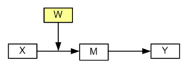
For this model there is an interaction between w and x
only in the mediator equation so we have to constrain the coefficient for the mediator
to be equal in both equations in addition to the covariate and residuals.
sem (0: m <- x cv@c1)(0: y <- m@b1 x cv@c2) ///
    (1: m <- x cv@c1)(1: y <- m@b1 x cv@c2), group(w) ///
    variance(0: e.m@v1 e.y@v2) ///
    variance(1: e.m@v1 e.y@v2)

Endogenous variables

Observed:  m y

Exogenous variables

Observed:  x cv

Fitting target model:

Iteration 0:   log likelihood = -2880.2553
Iteration 1:   log likelihood = -2814.5984
Iteration 2:   log likelihood =  -2797.118
Iteration 3:   log likelihood = -2796.3599
Iteration 4:   log likelihood = -2796.3547
Iteration 5:   log likelihood = -2796.3547

Structural equation model                       Number of obs      =       200
Grouping variable  = w                          Number of groups   =         2
Estimation method  = ml
Log likelihood     = -2796.3547

 ( 1)  [y]0bn.w#c.m - [y]1.w#c.m = 0
 ( 2)  [m]0bn.w#c.cv - [m]1.w#c.cv = 0
 ( 3)  [y]0bn.w#c.cv - [y]1.w#c.cv = 0
 ( 4)  [var(e.m)]0bn.w - [var(e.m)]1.w = 0
 ( 5)  [var(e.y)]0bn.w - [var(e.y)]1.w = 0
------------------------------------------------------------------------------
             |                 OIM
             |      Coef.   Std. Err.      z    P>|z|     [95% Conf. Interval]
-------------+----------------------------------------------------------------
Structural   |
  m <-       |
    x        |
        male |   .4525824   .0821032     5.51   0.000      .291663    .6135017
      female |   .5435942   .0815035     6.67   0.000     .3838503    .7033381
    cv       |
         [*] |   .3576463   .0548017     6.53   0.000     .2502369    .4650557
    _cons    |
        male |   10.33924   4.225914     2.45   0.014     2.056604    18.62188
      female |   4.326879   4.000738     1.08   0.279    -3.514423    12.16818
  -----------+----------------------------------------------------------------
  y <-       |
    m        |
         [*] |   .3384145   .0719076     4.71   0.000     .1974781    .4793508
    x        |
        male |   .4260495   .0896114     4.75   0.000     .2504144    .6016846
      female |   .3501396    .091638     3.82   0.000     .1705324    .5297469
    cv       |
         [*] |   .0503993   .0613771     0.82   0.412    -.0698976    .1706962
    _cons    |
        male |   10.18685   4.361284     2.34   0.020     1.638888    18.73481
      female |   12.17734   4.080339     2.98   0.003     4.180026    20.17466
-------------+----------------------------------------------------------------
Variance     |
  e.m        |
         [*] |   48.05346   4.805346                      39.50068    58.45812
  e.y        |
         [*] |   49.69406   4.969406                      40.84927    60.45394
------------------------------------------------------------------------------
Note: [*] identifies parameter estimates constrained to be equal across
      groups.
LR test of model vs. saturated: chi2(5)   =      7.16, Prob > chi2 = 0.2093

estat teffects

Direct effects
------------------------------------------------------------------------------
             |                 OIM
             |      Coef.   Std. Err.      z    P>|z|     [95% Conf. Interval]
-------------+----------------------------------------------------------------
Structural   |
  m <-       |
    x        |
        male |   .4525824   .0821032     5.51   0.000      .291663    .6135017
      female |   .5435942   .0815035     6.67   0.000     .3838503    .7033381
    cv       |
        male |   .3576463   .0548017     6.53   0.000     .2502369    .4650557
      female |   .3576463   .0548017     6.53   0.000     .2502369    .4650557
  -----------+----------------------------------------------------------------
  y <-       |
    m        |
        male |   .3384145   .0719076     4.71   0.000     .1974781    .4793508
      female |   .3384145   .0719076     4.71   0.000     .1974781    .4793508
    x        |
        male |   .4260495   .0896114     4.75   0.000     .2504144    .6016846
      female |   .3501396    .091638     3.82   0.000     .1705324    .5297469
    cv       |
        male |   .0503993   .0613771     0.82   0.412    -.0698976    .1706962
      female |   .0503993   .0613771     0.82   0.412    -.0698976    .1706962
------------------------------------------------------------------------------


Indirect effects
------------------------------------------------------------------------------
             |                 OIM
             |      Coef.   Std. Err.      z    P>|z|     [95% Conf. Interval]
-------------+----------------------------------------------------------------
Structural   |
  m <-       |
    x        |
         [*] |          0  (no path)
    cv       |
         [*] |          0  (no path)
  -----------+----------------------------------------------------------------
  y <-       |
    m        |
         [*] |          0  (no path)
    x        |
        male |   .1531604   .0427916     3.58   0.000     .0692904    .2370304
      female |   .1839601   .0478402     3.85   0.000     .0901952    .2777251
    cv       |
        male |   .1210327    .031707     3.82   0.000     .0588882    .1831772
      female |   .1210327    .031707     3.82   0.000     .0588882    .1831772
------------------------------------------------------------------------------
Note: [*] identifies parameter estimates constrained to be equal across
      groups.


Total effects
------------------------------------------------------------------------------
             |                 OIM
             |      Coef.   Std. Err.      z    P>|z|     [95% Conf. Interval]
-------------+----------------------------------------------------------------
Structural   |
  m <-       |
    x        |
        male |   .4525824   .0821032     5.51   0.000      .291663    .6135017
      female |   .5435942   .0815035     6.67   0.000     .3838503    .7033381
    cv       |
        male |   .3576463   .0548017     6.53   0.000     .2502369    .4650557
      female |   .3576463   .0548017     6.53   0.000     .2502369    .4650557
  -----------+----------------------------------------------------------------
  y <-       |
    m        |
        male |   .3384145   .0719076     4.71   0.000     .1974781    .4793508
      female |   .3384145   .0719076     4.71   0.000     .1974781    .4793508
    x        |
        male |     .57921   .0879948     6.58   0.000     .4067433    .7516766
      female |   .5340998    .087352     6.11   0.000     .3628929    .7053066
    cv       |
        male |    .171432   .0587342     2.92   0.004     .0563151    .2865488
      female |    .171432   .0587342     2.92   0.004     .0563151    .2865488
------------------------------------------------------------------------------
This time the indirect effect of x on y for males is .1531604 while
for females it is .1839601.
Next up is Model 3.
Model 3
Here is the diagram for Model 3.
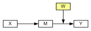
For Model 3 the interaction term is only in the equation for the dependent variable, y.
To compute the indirect effect we will need to constrain the coefficient for x in
both equations along with cv and the residuals. In addition we will need to
constrain the constant, _cons to be equal in both groups for the first equation.
sem (0: m <- x@b1 cv@c1 _cons@i1)(0: y <- m x@b2 cv@c2) ///
    (1: m <- x@b1 cv@c1 _cons@i1)(1: y <- m x@b2 cv@c2), group(w) ///
    variance(0: e.m@v1 e.y@v2) ///
    variance(1: e.m@v1 e.y@v2)

Endogenous variables

Observed:  m y

Exogenous variables

Observed:  x cv

Fitting target model:

Iteration 0:   log likelihood = -2809.2798
Iteration 1:   log likelihood =  -2797.463
Iteration 2:   log likelihood = -2796.0327
Iteration 3:   log likelihood = -2796.0196
Iteration 4:   log likelihood = -2796.0196

Structural equation model                       Number of obs      =       200
Grouping variable  = w                          Number of groups   =         2
Estimation method  = ml
Log likelihood     = -2796.0196

 ( 1)  [m]0bn.w#c.x - [m]1.w#c.x = 0
 ( 2)  [m]0bn.w#c.cv - [m]1.w#c.cv = 0
 ( 3)  [y]0bn.w#c.x - [y]1.w#c.x = 0
 ( 4)  [y]0bn.w#c.cv - [y]1.w#c.cv = 0
 ( 5)  [var(e.m)]0bn.w - [var(e.m)]1.w = 0
 ( 6)  [var(e.y)]0bn.w - [var(e.y)]1.w = 0
 ( 7)  [m]0bn.w - [m]1.w = 0
------------------------------------------------------------------------------
             |                 OIM
             |      Coef.   Std. Err.      z    P>|z|     [95% Conf. Interval]
-------------+----------------------------------------------------------------
Structural   |
  m <-       |
    x        |
         [*] |   .5038419   .0628899     8.01   0.000     .3805799    .6271038
    cv       |
         [*] |     .35414     .05488     6.45   0.000     .2465771    .4617029
    _cons    |
         [*] |   7.146537   3.017773     2.37   0.018     1.231809    13.06126
  -----------+----------------------------------------------------------------
  y <-       |
    m        |
        male |    .425432   .0861437     4.94   0.000     .2565935    .5942706
      female |   .2444712   .0863545     2.83   0.005     .0752194    .4137229
    x        |
         [*] |   .3979248   .0727133     5.47   0.000     .2554093    .5404402
    cv       |
         [*] |   .0489704   .0609254     0.80   0.422    -.0704413     .168382
    _cons    |
        male |    7.15329   4.182562     1.71   0.087     -1.04438    15.35096
      female |   14.60934    3.86371     3.78   0.000     7.036603    22.18207
-------------+----------------------------------------------------------------
Variance     |
  e.m        |
         [*] |    48.6004    4.86004                      39.95027    59.12348
  e.y        |
         [*] |   48.97042   4.897041                      40.25443    59.57361
------------------------------------------------------------------------------
Note: [*] identifies parameter estimates constrained to be equal across
      groups.
LR test of model vs. saturated: chi2(7)   =      6.49, Prob > chi2 = 0.4843

estat teffects

Direct effects
------------------------------------------------------------------------------
             |                 OIM
             |      Coef.   Std. Err.      z    P>|z|     [95% Conf. Interval]
-------------+----------------------------------------------------------------
Structural   |
  m <-       |
    x        |
        male |   .5038419   .0628899     8.01   0.000     .3805799    .6271038
      female |   .5038419   .0628899     8.01   0.000     .3805799    .6271038
    cv       |
        male |     .35414     .05488     6.45   0.000     .2465771    .4617029
      female |     .35414     .05488     6.45   0.000     .2465771    .4617029
  -----------+----------------------------------------------------------------
  y <-       |
    m        |
        male |    .425432   .0861437     4.94   0.000     .2565935    .5942706
      female |   .2444712   .0863545     2.83   0.005     .0752194    .4137229
    x        |
        male |   .3979248   .0727133     5.47   0.000     .2554093    .5404402
      female |   .3979248   .0727133     5.47   0.000     .2554093    .5404402
    cv       |
        male |   .0489704   .0609254     0.80   0.422    -.0704413     .168382
      female |   .0489704   .0609254     0.80   0.422    -.0704413     .168382
------------------------------------------------------------------------------


Indirect effects
------------------------------------------------------------------------------
             |                 OIM
             |      Coef.   Std. Err.      z    P>|z|     [95% Conf. Interval]
-------------+----------------------------------------------------------------
Structural   |
  m <-       |
    x        |
         [*] |          0  (no path)
    cv       |
         [*] |          0  (no path)
  -----------+----------------------------------------------------------------
  y <-       |
    m        |
         [*] |          0  (no path)
    x        |
        male |   .2143505   .0509868     4.20   0.000     .1144182    .3142827
      female |   .1231748   .0461456     2.67   0.008      .032731    .2136186
    cv       |
        male |   .1506625    .038416     3.92   0.000     .0753685    .2259565
      female |    .086577   .0333952     2.59   0.010     .0211236    .1520304
------------------------------------------------------------------------------
Note: [*] identifies parameter estimates constrained to be equal across
      groups.


Total effects
------------------------------------------------------------------------------
             |                 OIM
             |      Coef.   Std. Err.      z    P>|z|     [95% Conf. Interval]
-------------+----------------------------------------------------------------
Structural   |
  m <-       |
    x        |
        male |   .5038419   .0628899     8.01   0.000     .3805799    .6271038
      female |   .5038419   .0628899     8.01   0.000     .3805799    .6271038
    cv       |
        male |     .35414     .05488     6.45   0.000     .2465771    .4617029
      female |     .35414     .05488     6.45   0.000     .2465771    .4617029
  -----------+----------------------------------------------------------------
  y <-       |
    m        |
        male |    .425432   .0861437     4.94   0.000     .2565935    .5942706
      female |   .2444712   .0863545     2.83   0.005     .0752194    .4137229
    x        |
        male |   .6122752   .0745834     8.21   0.000     .4660944     .758456
      female |   .5210996   .0681111     7.65   0.000     .3876042     .654595
    cv       |
        male |   .1996329   .0622773     3.21   0.001     .0775716    .3216941
      female |   .1355474   .0595838     2.27   0.023     .0187652    .2523295
------------------------------------------------------------------------------
This time the indirect effect of x on y for males is .2143505 while
for females it is .1231748.