
It is not uncommon to believe a variable x predicts a variable y
differently over certain ranges of x. In such instances, you may
wish to fit a piecewise regression model. The simplest scenario
would be fitting two adjoined lines: one line defines the relationship of y
and x for x <= c and the other line defines the
relationship for x > c. For this scenario, we can use the
Stata command
nl to find the value of c that yields the best fitting model.
The nl command in Stata performs nonlinear least-squares estimation and
allows the user to define the function for which it estimates indicated
parameters. It is extremely flexible and very useful, though slightly tricky to
use at first. The page presents a rather simple example. For details
and more examples on nl, see its Stata help page.
For this example, we will use a fictional dataset where the relationship
between x and y is clearly not a single line.
use https://stats.oarc.ucla.edu/wp-content/uploads/2022/07/nl.dta, clear
twoway scatter y x
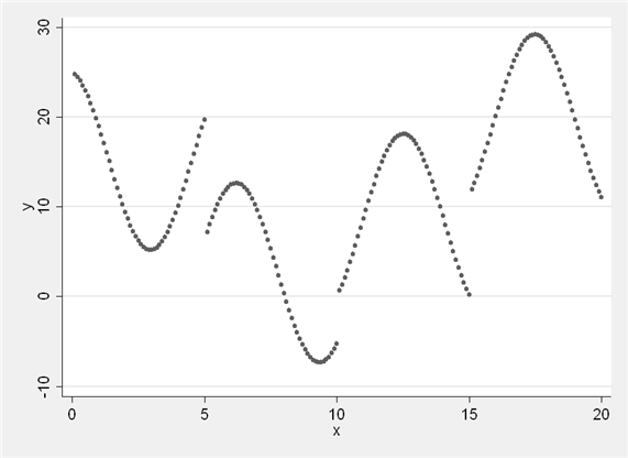
We might look at this plot and
believe that there is a downward trend in y as x increases up to a
certain point in x. After that point, there is an upward trend in
y. Let’s consider the set of parameters we will need to fit.
Our first line will involve a slope and an intercept (a1 and b1);
our second line will also involve a slope (b2) and we can think of the
point at which it meets the first line as its “intercept” defined by the first
intercept, the first slope, and the point at which the lines meet (c). We want to
estimate four total parameters: two slopes, an intercept, and a cut point.
We can indicate these parameters in our nl command and provide starting points for
each parameter based on the plot above.
nl (y = ({a1} + {b1}*x)*(x < {c}) + ///
	  ({a1} + {b1}*{c} + {b2}*(x-{c}))*(x >= {c})), ///
	   initial(a1 25 b1 -2 c 10 b2 2)

      Source |       SS       df       MS
-------------+------------------------------         Number of obs =       200
       Model |  8770.59791     3  2923.53264         R-squared     =    0.5169
    Residual |  8197.31882   196  41.8230552         Adj R-squared =    0.5095
-------------+------------------------------         Root MSE      =  6.467075
       Total |  16967.9167   199  85.2659132         Res. dev.     =  1310.224

------------------------------------------------------------------------------
           y |      Coef.   Std. Err.      t    P>|t|     [95% Conf. Interval]
-------------+----------------------------------------------------------------
         /a1 |   18.53111   1.382652    13.40   0.000     15.80433     21.2579
         /b1 |  -1.920463   .2668338    -7.20   0.000    -2.446697   -1.394229
          /c |   8.987615   .4400011    20.43   0.000      8.11987    9.855359
         /b2 |   2.267615   .1915718    11.84   0.000     1.889808    2.645422
------------------------------------------------------------------------------
  Parameter a1 taken as constant term in model & ANOVA table
From the output above, we can see estimates of all four
parameters. We can use the estimate for the cut point c to generate
a new variable, x2, that will allow us to run an ordinary least squares
regression of y on x and x2 that effectively fits a
piecewise function.
gen x2 = x - 8.987615
replace x2 = 0 if x < 8.987615

regress y x x2

      Source |       SS       df       MS              Number of obs =     200
-------------+------------------------------           F(  2,   197) =  105.39
       Model |  8770.59777     2  4385.29889           Prob > F      =  0.0000
    Residual |  8197.31896   197  41.6107562           R-squared     =  0.5169
-------------+------------------------------           Adj R-squared =  0.5120
       Total |  16967.9167   199  85.2659132           Root MSE      =  6.4506

------------------------------------------------------------------------------
           y |      Coef.   Std. Err.      t    P>|t|     [95% Conf. Interval]
-------------+----------------------------------------------------------------
           x |  -1.920463   .2023035    -9.49   0.000    -2.319422   -1.521505
          x2 |   4.188078   .3214448    13.03   0.000     3.554163    4.821993
       _cons |   18.53111   1.275748    14.53   0.000     16.01524    21.04699
------------------------------------------------------------------------------
In the regression output, we can see that we have the same sum of
squares we saw in the nl output. We also see that our intercept is
unchanged (a1 in the nl output, _cons in the regress
output), the coefficient for x matches the first slope from nl, and the coefficient for x2 is equal to (b2 – b1).
We can plot the predicted values from the regression above.
predict p
graph twoway (scatter y x) (scatter p x)
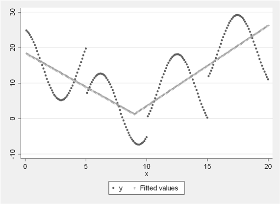
We have found the optimal point to split our piecewise function in this
scenario. The same process could be used if we wished to fit quadratic or
cubic terms, as long as we carefully described the function and its parameters
in our nl command.