Seminar HLM 6.08 – OARC Stats

This seminar covers the basics of two-level hierarchical linear models using
HLM 6.08. We will use
data files from the High School and Beyond Survey. The data files in SPSS format
come with HLM software and are located in the subfolder /examples/Chpater2 of
the HLM
folder.

Outline

Getting data into the HLM program
- ASCII files
- files from common statistical packages
The data set
- description of example data set and where to find it
- a brief word about sample size
Model building
- unconditional means model
- regression with means-as-outcomes
- random-coefficient model
- intercepts and slopes-as-outcomes model
- graphing the results
Model fit
- model checking based on the residual file
- testing homogeneity of level-1 variances
- multivariate hypothesis tests of fixed effects
- multivariate tests of variance-covariance components specification
Other issues
- modeling heterogeneity of level-1 variances
- models without a level-1 intercept
- constraints of fixed effects
- testing multi-degree-of-freedom variables
- using probability weights
- multiply imputed data files

Getting data into HLM

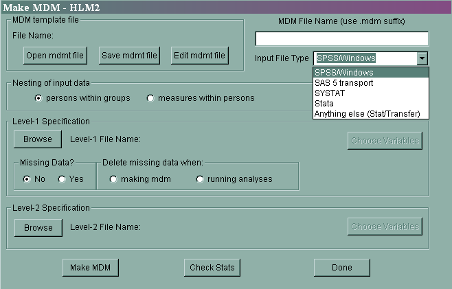
Getting data into HLM 6.08 is much easier than it was in earlier versions.
Previously, the data for the level 1 variables had to be in one data file, and the
variables for level 2 had to be in a different data file. Now, both level
1 and level 2 variables can be in the same data file. It is very easy to
bring in SPSS, SAS and Stata (including version 11) data files using the Input File Type pull-down
menu.

Missing data are often an issue with multilevel data. HLM will allow
missing values at level 1, but it will not allow missing values at level 2.
If you have missing data at level 2, you will want to remove those cases before
you bring your data into HLM. Alternatively, if you have multiply
imputed data files, you can use those. A brief example will be shown
at the end of the seminar.

The data set

Our data file is a subsample from the 1982 High School and Beyond Survey and
is used extensively in Hierarchical Linear Models by Raudenbush and Bryk.
The data file, called hsb, consists of 7185 students nested in 160 schools. The outcome
variable of interest is the student-level (level 1) math achievement score (mathach).
The variable ses is the socio-economic status of a student and therefore is at
the student level. The variable meanses is the group-mean centered
version of ses
and therefore is at the school level (level 2). The variable sector
is an indicator variable indicating if a school is public or catholic and is
therefore a school-level variable. There are 90 public schools (sector=0) and 70
catholic schools (sector=1) in the sample.

The file that we are going to use is located in Chapter 2 in the Examples
folder in your HLM
folder and is called hsb1.sav and hsb2.sav (C:Program FilesHLM6ExamplesChapter2hsb1.sav and

C:Program
FilesHLM6ExamplesChapter2hsb2.sav).

A brief word about sample sizes

The sample size necessary for multilevel modeling depends on several factors,
including the number of parameters being estimated, the intraclass correlation,
how balanced the data are, and some other things. In general, however,
multilevel modeling
is a large sample procedure. In particular, you usually want to have as
many level 2 units as possible. Having lots of level 1 units can be
helpful, but remember that level 1 units are correlated within each level 2 unit
(the intraclass correlation), so increasing the number of level 1 units can
become a case of diminishing returns. Level 2 units are independent (in a
two level model), so by increasing the number of level 2 units, you are adding
additional pieces of independent information to the data set. The validity
of inferences made from small sample sizes is discussed in Hierarchical Linear Models by Raudenbush and Bryk
on pages 280-284. Information regarding samples sizes can also be found in
Snijders and Bosker’s Multilevel Analysis. Some of the references
listed at the end of this page also contain information regarding sample sizes.

Model building

At this point, we will focus on modeling building using HLM. We will pretend that
we have already done data cleaning and have created all necessary variables.
We will also assume that we have successfully gotten our data into HLM.
For each of the models that we create, we will show both the model to be
estimated in both the multi-equation and the single (mixed) equation format.
The multi-equation format is shown by default; you can see the mixed equation by
clicking on the mixed button in the lower left corner of the HLM interface.

Model 1: Unconditional means model

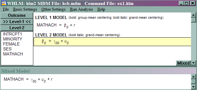
This model is referred as a one-way random effect ANOVA and is the
simplest possible random effect linear model. The motivation for this model is
the question of how much schools vary in their mean mathematics
achievement. In terms of equations, we have the following, where r_ij
~ N(0, σ²) and u_0j~ N(0, τ²),

mathach_ij= β_0j+ r_ij

β_0j= γ₀₀+ u_0j

  SPECIFICATIONS FOR THIS HLM2 RUN

  Problem Title: no title

  The data source for this run  = hsb.mdm
  The command file for this run = C:Datadataex1.hlm
  Output file name              = c:hlm2.txt
  The maximum number of level-1 units = 7185
  The maximum number of level-2 units = 160
  The maximum number of iterations = 100
  Method of estimation: restricted maximum likelihood

 Weighting Specification
 -----------------------
                         Weight
                         Variable
            Weighting?   Name        Normalized?
 Level 1        no       
 Level 2        no       
 Precision      no       

  The outcome variable is  mathach    

  The model specified for the fixed effects was:
 ----------------------------------------------------

   Level-1                  Level-2
   Coefficients             Predictors
 ----------------------   ---------------
         intrcpt1, B0      INTRCPT2, G00   

 The model specified for the covariance components was:
 ---------------------------------------------------------

         Sigma squared (constant across level-2 units)

         Tau dimensions
               intrcpt1

 Summary of the model specified (in equation format)
 ---------------------------------------------------

Level-1 Model

	Y = B0 + R

Level-2 Model
	B0 = G00 + U0

Iterations stopped due to small change in likelihood function
******* ITERATION 4 *******

 Sigma_squared =     39.14831

 Tau
 intrcpt1,B0      8.61431 


Tau (as correlations)
 intrcpt1,B0  1.000

 ----------------------------------------------------
  Random level-1 coefficient   Reliability estimate
 ----------------------------------------------------
  intrcpt1, B0                        0.901
 ----------------------------------------------------

The value of the likelihood function at iteration 4 = -2.355840E+004
The outcome variable is  mathach

 Final estimation of fixed effects:
 ----------------------------------------------------------------------------
                                       Standard             Approx.
    Fixed Effect         Coefficient   Error      T-ratio   d.f.     P-value
 ----------------------------------------------------------------------------
 For       intrcpt1, B0
    INTRCPT2, G00          12.636972   0.244412    51.704       159    0.000
 ----------------------------------------------------------------------------

 The outcome variable is  mathach

 Final estimation of fixed effects
 (with robust standard errors)
 ----------------------------------------------------------------------------
                                       Standard             Approx.
    Fixed Effect         Coefficient   Error      T-ratio   d.f.     P-value
 ----------------------------------------------------------------------------
 For       intrcpt1, B0
    INTRCPT2, G00          12.636972   0.243628    51.870       159    0.000
 ----------------------------------------------------------------------------

 Final estimation of variance components:
 -----------------------------------------------------------------------------
 Random Effect           Standard      Variance     df    Chi-square  P-value
                         Deviation     Component
 -----------------------------------------------------------------------------
 intrcpt1,       U0        2.93501       8.61431   159    1660.23259    0.000
  level-1,       R         6.25686      39.14831
 -----------------------------------------------------------------------------

 Statistics for current covariance components model
 --------------------------------------------------
 Deviance                       = 47116.793477
 Number of estimated parameters = 2

Notes:

The model we fit was
mathach_ij= β_0j+ r_ij

β_0j= γ₀₀+ u_0j

Filling in the parameter estimates we get

mathach_ij= β_0j+ r_ij

β_0j= 12.64+ u_0jV(u_0j) = 8.61
V(r_ij) = 39.15
The estimated between variance, τ²,
corresponds to the term intrcpt1 in the output of final estimation of
variance components and the estimated within variance, σ²,
corresponds to the term level-1 in the same output section. For this
model, τ² is 8.61 and σ² is 39.15.
Based on the covariance estimates, we can compute the intraclass
correlation: 8.61431/(8.61431 + 39.14831) = .18. This tells us the
portion of the total variance that occurs between schools.
To measure the magnitude of the variation among schools in their mean
achievement levels, we can calculate the plausible values range for
these means, based on the between variance we obtained from the model: 12.64
± 1.96*(8.61)^1/2 = (6.89,
18.39).
The reliability of the random effect of the level 1 intercept is the
average reliability of the level 2 units. It measures the overall reliability
of the OLS estimates for each of the intercepts. The reliability estimate
for this model is .901.

Model 2: Including effects of school level (level 2) predictors –
predicting mathach from meanses

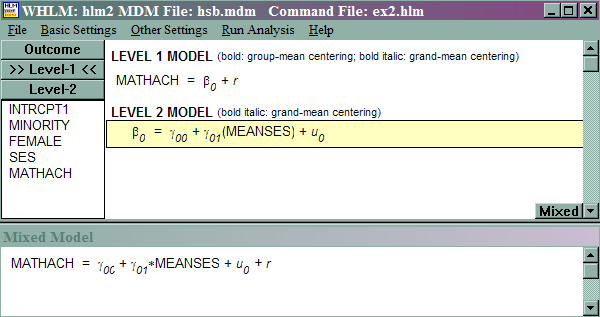
This model is referred to as regression with means-as-outcomes by Raudenbush and
Bryk. This model is motivated by the question of whether schools with high
meanses also have high math achievement. In other words, we want to
understand why there is a school difference with regard to mathematics
achievement. In terms of regression equations, we have the following:

mathach_ij= β_0j+ r_ij

β_0j= γ₀₀+ γ₀₁(meanses)
+ u_0j

 SPECIFICATIONS FOR THIS HLM2 RUN

  Problem Title: no title

  The data source for this run  = hsb.mdm
  The command file for this run = C:Datadataex2.hlm
  Output file name              = c:hlm2.txt
  The maximum number of level-1 units = 7185
  The maximum number of level-2 units = 160
  The maximum number of iterations = 100
  Method of estimation: restricted maximum likelihood

 Weighting Specification
 -----------------------
                         Weight
                         Variable
            Weighting?   Name        Normalized?
 Level 1        no       
 Level 2        no       
 Precision      no       

  The outcome variable is  mathach    

  The model specified for the fixed effects was:
 ----------------------------------------------------

   Level-1                  Level-2
   Coefficients             Predictors
 ----------------------   ---------------
         intrcpt1, B0      INTRCPT2, G00   
                            meanses, G01   

 The model specified for the covariance components was:
 ---------------------------------------------------------

         Sigma squared (constant across level-2 units)

         Tau dimensions
               intrcpt1

 Summary of the model specified (in equation format)
 ---------------------------------------------------

Level-1 Model

	Y = B0 + R

Level-2 Model
	B0 = G00 + G01*(meanses) + U0

Iterations stopped due to small change in likelihood function
******* ITERATION 6 *******

 Sigma_squared =     39.15708

 Tau
 intrcpt1,B0      2.63870 

Tau (as correlations)
 intrcpt1,B0  1.000

 ----------------------------------------------------
  Random level-1 coefficient   Reliability estimate
 ----------------------------------------------------
  intrcpt1, B0                        0.740
 ----------------------------------------------------

The value of the likelihood function at iteration 6 = -2.347972E+004
The outcome variable is  mathach

 Final estimation of fixed effects:
 ----------------------------------------------------------------------------
                                       Standard             Approx.
    Fixed Effect         Coefficient   Error      T-ratio   d.f.     P-value
 ----------------------------------------------------------------------------
 For       intrcpt1, B0
    INTRCPT2, G00          12.649436   0.149280    84.736       158    0.000
     meanses, G01           5.863538   0.361457    16.222       158    0.000
 ----------------------------------------------------------------------------

 The outcome variable is  mathach

 Final estimation of fixed effects
 (with robust standard errors)
 ----------------------------------------------------------------------------
                                       Standard             Approx.
    Fixed Effect         Coefficient   Error      T-ratio   d.f.     P-value
 ----------------------------------------------------------------------------
 For       intrcpt1, B0
    INTRCPT2, G00          12.649436   0.148377    85.252       158    0.000
     meanses, G01           5.863538   0.320211    18.311       158    0.000
 ----------------------------------------------------------------------------

 Final estimation of variance components:
 -----------------------------------------------------------------------------
 Random Effect           Standard      Variance     df    Chi-square  P-value
                         Deviation     Component
 -----------------------------------------------------------------------------
 intrcpt1,       U0        1.62441       2.63870   158     633.51744    0.000
  level-1,       R         6.25756      39.15708
 -----------------------------------------------------------------------------

 Statistics for current covariance components model
 --------------------------------------------------
 Deviance                       = 46959.446959
 Number of estimated parameters = 2

Notes:

The model we fit was
mathach_ij= β_0j+ r_ij

β_0j= γ₀₀+ γ₀₁(meanses)
+ u_0j

Filling in the parameter
estimates we get

mathach_ij= β_0j+ r_ij

β_0j= 12.65 +5.86(meanses)
+ u_0jV(u_0j) = 2.64V(r_ij) = 39.16
In a single equation our model will be written as: mathach_ij=
γ₀₀+ γ₀₁(meanses)
+ u_0j+ r_ij.
The coefficient for the constant is the predicted math achievement when
all predictors are 0; hence, when the average school SES is 0, the students’ math
achievement is predicted to be 12.65.
A range of plausible values for school means, given that all schools have
meanses of zero, is 12.65 ± 1.96 *(2.64)^1/2
= (9.47, 15.83).
The variance component representing variation between schools decreases
greatly (from 8.61 to 2.64). This indicates that the level-2 variable
meanses explains a large portion of the school-to-school variation in mean
math achievement. More precisely, the proportion of variance explained by
meanses is (8.61 – 2.64)/8.61 = .69, that is about 69% of the explainable
variation in school mean math achievement scores can be explained by
meanses.
Do school achievement means still vary
significantly once meanses is controlled? The output of final estimation of
variance components gives the test for the variance component for the intrcpt1
to be zero with chi-square of 633.52 with 158 degrees of freedom. This is
statistically
significant. Therefore, we conclude that after controlling for meanses,
significant variation among school mean math achievement still remains to be
explained.
We can also calculate the conditional
intraclass correlation conditional on the values of meanses: 2.64/(2.64 +
39.16) = .06 measures the degree of dependence among observations within
schools that are of the same meanses.

Model 3: Including effects of student-level predictors-predicting
mathach from group–centered student-level ses

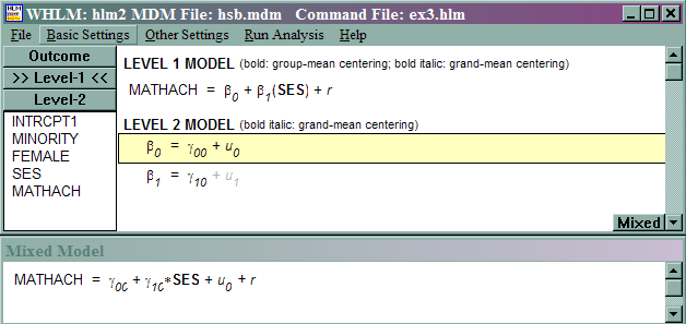
This model is referred to as a random-coefficient model by Raudenbush and Bryk.
Pretend that we run a regression of mathach on group-centered ses
for
each school; in other words, we would run 160 regressions.

What would be the average of the 160 regression equations (both intercept
and slope)?
How much do the regression equations vary from school to school?
What is the correlation between the intercepts and slopes?

These are some of the questions that motivates the following model.

mathach_ij= β_0j+ β_1j
(SES – meanses) + r_ij
β_0j= γ₀₀ + u_0jβ_1j= γ₁₀ + u_1j

 Sigma_squared =     36.70356

 Tau
 intrcpt1,B0      8.68087       0.04701 
      SES,B1      0.04701       0.68038

Tau (as correlations)
 intrcpt1,B0  1.000  0.019
      SES,B1  0.019  1.000

 ----------------------------------------------------
  Random level-1 coefficient   Reliability estimate
 ----------------------------------------------------
  intrcpt1, B0                        0.908
       SES, B1                        0.260
 ----------------------------------------------------

The value of the likelihood function at iteration 18 = -2.335620E+004

 Final estimation of fixed effects:
 ----------------------------------------------------------------------------
                                       Standard             Approx.
    Fixed Effect         Coefficient   Error      T-ratio   d.f.     P-value
 ----------------------------------------------------------------------------
 For       intrcpt1, B0
    INTRCPT2, G00          12.636197   0.244503    51.681       159    0.000
 For      SES slope, B1
    INTRCPT2, G10           2.193157   0.127879    17.150       159    0.000
 ----------------------------------------------------------------------------

 Final estimation of fixed effects
 (with robust standard errors)
 ----------------------------------------------------------------------------
                                       Standard             Approx.
    Fixed Effect         Coefficient   Error      T-ratio   d.f.     P-value
 ----------------------------------------------------------------------------
 For       intrcpt1, B0
    INTRCPT2, G00          12.636197   0.243738    51.843       159    0.000
 For      SES slope, B1
    INTRCPT2, G10           2.193157   0.127846    17.155       159    0.000
 ----------------------------------------------------------------------------

 Final estimation of variance components:
 -----------------------------------------------------------------------------
 Random Effect           Standard      Variance     df    Chi-square  P-value
                         Deviation     Component
 -----------------------------------------------------------------------------
 intrcpt1,       U0        2.94633       8.68087   159    1770.85120    0.000
      SES slope, U1        0.82485       0.68038   159     213.43769    0.003
  level-1,       R         6.05835      36.70356
 -----------------------------------------------------------------------------

 Statistics for current covariance components model
 --------------------------------------------------
 Deviance                       = 46712.398925
 Number of estimated parameters = 4

Notes:

The model we fit was
mathach_ij= β_0j+ β_1j
(SES – meanses) + r_ij
β_0j= γ₀₀ + u_0jβ_1j= γ₁₀ + u_1j

Filling in the parameter
estimates we get

mathach_ij= β_0j+ β_1j
(SES – meanses) + r_ij
β_0j= 12.64 + u_0jβ_1j= 2.19 + u_1j
V(u_0j) = 8.68
V(u_1j) = .68
V(r_ij) = 36.7
In a single equation our model would be written as:
mathach_ij=
γ₀₀ + u_0j+ (γ₁₀ + u_1j )(SES – meanses) + r_{ij

=}
γ₀₀ + γ₁₀*(SES –
meanses) +
u_0j+ u_1j *(SES – meanses) + r_ij
The estimate for the variance of the slope for group-centered SES is
0.68. The p-value is .003. Because the test is statistically significant, we
reject the hypothesis that there is no difference in slopes among schools.
The 95% plausible value range for the school means is 12.64
± 1.96 *(8.68)^1/2 = (6.87, 18.41).
The 95% plausible value range for the
SES-achievement slope is 2.19 ± 1.96
*(.68)^1/2 = (.57, 3.81).
Notice that the residual variance is now
36.70, compared to the residual variance of 39.15 in the one-way ANOVA with
random effects (unconditional means) model. We can compute the proportion variance explained at
level 1 as (39.15 – 36.70) / 39.15 = .063. This suggests using student-level SES
as a predictor of math achievement reduced the within-school variance by 6.3%.
The correlation between the intercept and the
slope is .019. It seems that they are not highly correlated.

Model 4: Including both level-1 and level-2 predictors -predicting
mathach from meanses, sector, cses and the cross level interaction of meanses and sector with cses

This model is referred to as an intercepts- and slopes-as-outcomes model by Raudenbush and Bryk. We have examined the variability of the regression
equations across schools. Now we will build an explanatory model to account for
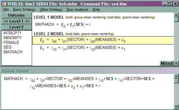
the variability. We want to model the following:

mathach_ij= β_0j+ β_1j
(SES – meanses) + r_ij
β_0j= γ₀₀ + γ₀₁(sector)
+ γ₀₂(meanses) + u_0jβ_1j= γ₁₀ + γ₁₁(sector) + γ₁₂(meanses)
+ u_1j

  SPECIFICATIONS FOR THIS HLM2 RUN

  Problem Title: no title

  The data source for this run  = hsb.mdm
  The command file for this run = C:Datadataex4.hlm
  Output file name              = c:hlm2.txt
  The maximum number of level-1 units = 7185
  The maximum number of level-2 units = 160
  The maximum number of iterations = 100
  Method of estimation: restricted maximum likelihood

 Weighting Specification
 -----------------------
                         Weight
                         Variable
            Weighting?   Name        Normalized?
 Level 1        no       
 Level 2        no       
 Precision      no       

  The outcome variable is  mathach    

  The model specified for the fixed effects was:
 ----------------------------------------------------

   Level-1                  Level-2
   Coefficients             Predictors
 ----------------------   ---------------
         intrcpt1, B0      INTRCPT2, G00   
                             SECTOR, G01   
                            meanses, G02   
 *      SES slope, B1      INTRCPT2, G10   
                             SECTOR, G11   
                            meanses, G12   

'*' - This level-1 predictor has been centered around its group mean.

 The model specified for the covariance components was:
 ---------------------------------------------------------

         Sigma squared (constant across level-2 units)

         Tau dimensions
               intrcpt1
                    SES slope


 Summary of the model specified (in equation format)
 ---------------------------------------------------

Level-1 Model

	Y = B0 + B1*(SES) + R

Level-2 Model
	B0 = G00 + G01*(SECTOR) + G02*(meanses) + U0
	B1 = G10 + G11*(SECTOR) + G12*(meanses) + U1

Iterations stopped due to small change in likelihood function
******* ITERATION 61 *******

 Sigma_squared =     36.70313

 Tau
 intrcpt1,B0      2.37996       0.19058 
      SES,B1      0.19058       0.14892 

Tau (as correlations)
 intrcpt1,B0  1.000  0.320
      SES,B1  0.320  1.000

 ----------------------------------------------------
  Random level-1 coefficient   Reliability estimate
 ----------------------------------------------------
  intrcpt1, B0                        0.733
       SES, B1                        0.073
 ----------------------------------------------------

The value of the likelihood function at iteration 61 = -2.325094E+004
The outcome variable is  mathach

 Final estimation of fixed effects:
 ----------------------------------------------------------------------------
                                       Standard             Approx.
    Fixed Effect         Coefficient   Error      T-ratio   d.f.     P-value
 ----------------------------------------------------------------------------
 For       intrcpt1, B0
    INTRCPT2, G00          12.096006   0.198734    60.865       157    0.000
      SECTOR, G01           1.226384   0.306272     4.004       157    0.000
     meanses, G02           5.333056   0.369161    14.446       157    0.000
 For      SES slope, B1
    INTRCPT2, G10           2.937981   0.157135    18.697       157    0.000
      SECTOR, G11          -1.640954   0.242905    -6.756       157    0.000
     meanses, G12           1.034427   0.302566     3.419       157    0.001
 ----------------------------------------------------------------------------

 The outcome variable is  mathach

 Final estimation of fixed effects
 (with robust standard errors)
 ----------------------------------------------------------------------------
                                       Standard             Approx.
    Fixed Effect         Coefficient   Error      T-ratio   d.f.     P-value
 ----------------------------------------------------------------------------
 For       intrcpt1, B0
    INTRCPT2, G00          12.096006   0.173699    69.638       157    0.000
      SECTOR, G01           1.226384   0.308484     3.976       157    0.000
     meanses, G02           5.333056   0.334600    15.939       157    0.000
 For      SES slope, B1
    INTRCPT2, G10           2.937981   0.147620    19.902       157    0.000
      SECTOR, G11          -1.640954   0.237401    -6.912       157    0.000
     meanses, G12           1.034427   0.332785     3.108       157    0.003
 ----------------------------------------------------------------------------

 Final estimation of variance components:
 -----------------------------------------------------------------------------
 Random Effect           Standard      Variance     df    Chi-square  P-value
                         Deviation     Component
 -----------------------------------------------------------------------------
 intrcpt1,       U0        1.54271       2.37996   157     605.29503    0.000
      SES slope, U1        0.38590       0.14892   157     162.30867    0.369
  level-1,       R         6.05831      36.70313
 -----------------------------------------------------------------------------

 Statistics for current covariance components model
 --------------------------------------------------
 Deviance                       = 46501.875643
 Number of estimated parameters = 4

Notes:

The model we fit was
mathach_ij= β_0j+ β_1j
(ses – meanses) + r_ij
β_0j= γ₀₀ + γ₀₁(sector)
+ γ₀₂(meanses) + u_0jβ_1j= γ₁₀ + γ₁₁(sector) + γ₁₂(meanses)
+ u_1j

Filling in the parameter
estimates we get

mathach_ij= β_0j+ β_1j
(ses – meanses) + r_ij
β_0j= 12.10 +
1.22(sector) + 5.33(meanses) + u_0jβ_1j= 2.94 + -1.64(sector) + 1.03(meanses)
+ u_1j

V(u_0j) = 2.37
V(u_1j) = .15
V(r_ij) = 36.7
In a single equation our model will be written as:
mathach_ij=
γ₀₀ + γ₀₁(meanses)
+ γ₀₂(sector) + u_0j+ (γ₁₀ + γ₁₁(meanses) + γ₁₂(sector)
+ u_1j)*
(ses – meanses) + r_ij

=
γ₀₀ + γ₀₁(meanses)
+ γ₀₂(sector)
                        +
γ₁₀*(ses-meanses) + γ₁₁*meanses*(ses-meanses) + γ_12*sector*(ses-meanses)

+ u_0j+ u_1j* (SES – meanses) + r_ij
The estimate for the variance of the ses slope is .15 with p-value .369;
hence, we fail to reject the null hypothesis that there is no significant variation among the
slopes of ses. We may want to use a simpler model where the
slope of ses varies nonrandomly with respect to the level-2 variables
meanses and
sector.
The correlation between the level-1 intercept and the slope for ses is
given as .32 from the earlier part of the output.

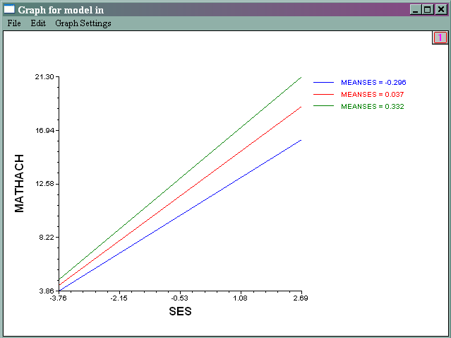
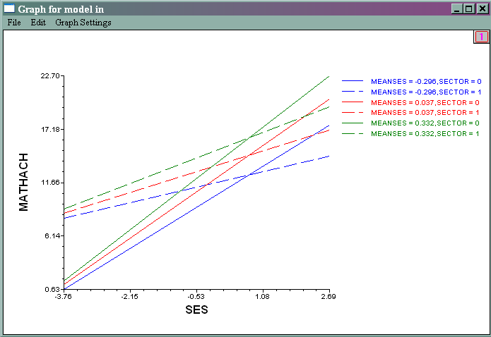
Graphing the results

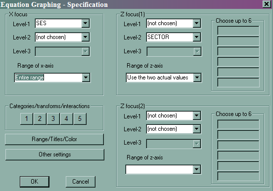
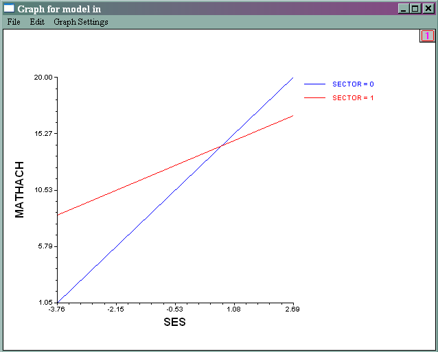
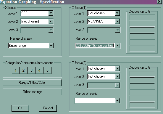
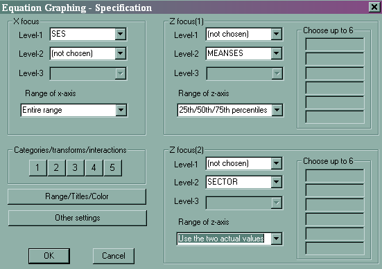
HLM has some nice features to help you visualize the effect of level 2 variables. After
running the model, you can click on File, and then Graph Equations and then
Model Graphs. All of the graphs in this section are based on the last
model that we ran, which we called model 4.

File -> Graph Equations -> Model Graphs
Slope of ses by sector
File -> Graph Equations -> Model Graphs
Slope of SES by different meanses
File -> Graph Equations -> Model Graphs
Putting the two plots together

Model fit

Residual file and analysis of model fit

Let’s say that our final model is going to be based on the
last model we ran with both the intercept and the slope for ses as random
effects. What about the model fit? Are there any potential problems with the
model?

Any outliers or influential observations?
Any omitted variables?
Normality at each level?
Homogeneity of level-1 variances?

1. Residual file

We can make use of the residual file that HLM creates to check model fit.
This time before running the model, we will request that a file of residuals be
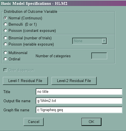
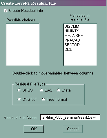
created. From the Basic Settings, click on Level-2 Residual File
and the following dialog window will be displayed. We can choose to include
in the file extra level-2 variables that are not in the model, and we can also choose the
residual file type. We will include variables in addition to our two level-2 variables in the
residual file, and we will request that the residual file be created in SPSS
format. All the plots and analyses based on the residual file will be preformed
in SPSS. You need to rerun the model after you specify what you want in
the residual file. You can include a path specification along with the file
name.

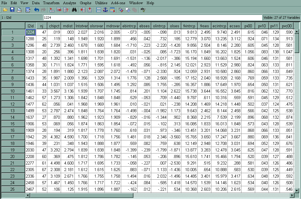
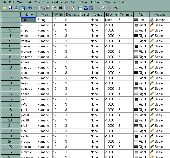
Let’s have a look at the residual file for our model. The last
six variables are all the level-2 variables in the file, and we have requested to
have them in the residual file. Each observation corresponds to a level-2 unit.
In our case, there will be 160 observations in the residual file, because there
are 160 schools.

l2id – Level-2 identification variable
nj – Size of the current level-2 unit
chipct – Theoretical values from a χ²(v)
with v being the number of random factors and this variable is paired with
mdist
to produce a Q-Q plot
mdist – Mahalanobis distance; under the normality assumption, it should be
approximately χ²(v) with v
being the number of random factors. It provides a summary measure of the
distance of the empirical Bayes estimates of the fixed effect parameters
from their "fitted value" given by our defining equations.
lntotvar – Natural log of the total dispersion within each level-2 unit
olsrsvar – Natural log of the residual dispersion within each level-2 unit
based on its OLS estimate
mdrsvar – Natural log of the residual standard deviation from the final
fitted fixed effect model
ebintrcp – Empirical Bayes residual for the intercept,
u_0j
ebses – Empirical Bayes residual for the slope of SES,
u_1j
olintrcp – Ordinary least square residual for the intercept, only for the
units with enough data
olses – Ordinary least square residual for the slope of SES, only for the
units with enough data
fvintrcp – Fitted value for the intercept based on its level-2 estimators,
β_0j.For example, for school id
1224, it is equal to12.096006 + 1.226384* 0 +
5.333056*(-.428) = 9.814
fvses – Fitted value for the slope of SES based on its level-2 estimators,
β_1j
pv00 – Posterior variance of the empirical Bayes estimate for the
intercept
pv10 – Posterior covariance of the empirical Bayes estimate for the
intercept and SES
pv11 – Posterior variance of the empirical Bayes estimate for the slope
pvc00 – Posterior variance of the coefficient for the random
intercept
pvc10 – Posterior covariance of the coefficients for the random
intercept and random slope
pvc11 – Posterior variance of the coefficient for the random
slope
size – Level 2 predictor variable from the original data file
pracad – Level 2 predictor variable from the original data file
disclim – Level 2 predictor variable from the original data file
himinity – Level 2 predictor variable from the original data file
sector – Level 2 predictor variable from the original data file
meanses – Level 2 predictor variable from the original data file

Q-Q Plot of chipct against mdist (Scatterplot of chipct against mdist)

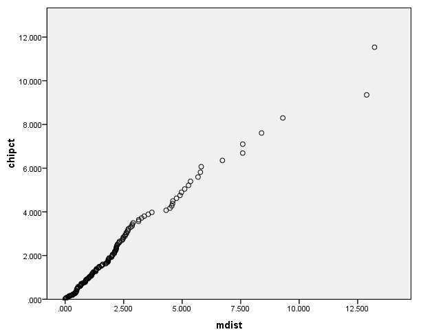
Under the assumption of normality at level-2, the plot of chipct against
mdist
should be a 45 degree line. Otherwise, we have some evidence against the
normality assumption. For example, in our plot we see some deviation from the
normality at the right end of the plot. The plot shows us that there may be some
outliers that need further investigation.

Histogram of mdrsvar

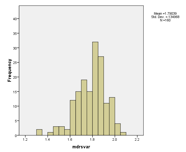
The variable mdrsvar (the natural log of the residual standard
deviation from the final fitted fixed effect model) measures the within-school standard deviation for
the 160 schools based on the final fitted model. From the histogram we see that
there are a few schools that have smaller within-school variance than others.

Q-Q Plot of standardized mdrsvar

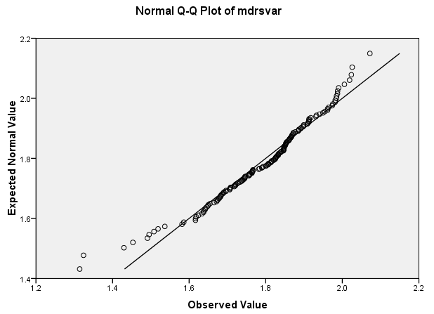
The purpose of this plot is similar to the previous one. If the data
are normally distributed, the dots will fall along the line. The
dots towards the left and right of the graph fall away from the line,
indicating that there is some divergence from normality in the tails of the
distribution.

Potential level-2 predictors

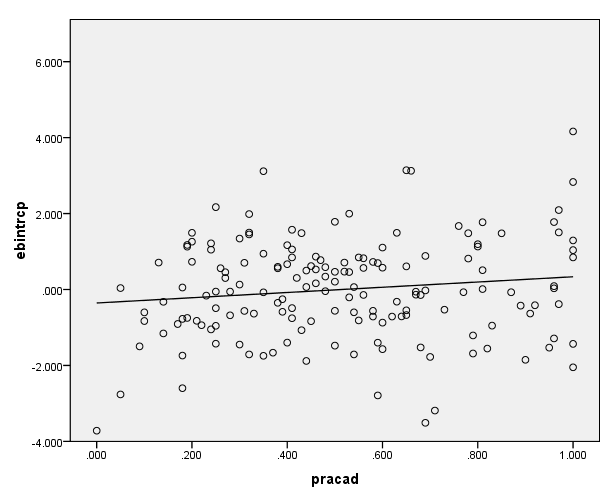
Potentially, there are other level-2 variables that should be included in the model.
(These other variables may or may not be in your data set.) For example, the variable
pracad, the proportion of students in the academic track,
may be a good candidate as a level-2 variable. To help visualize this, we can plot
the empirical Bayes residual estimate for the intercept for each school against
pracad.
The evidence that there is not much of an association between the intercept
and pracad suggests that this variable should not be included in the
model unless there is good theoretical reason to include it. All the same, we may have a model specification error, meaning we
have omitted one or more important variables.

Nonlinearity at level-2

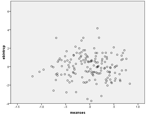
This is very similar to what we usually do in an OLS analysis. We plot the
residual against a continuous predictor to detect any nonlinearity. In this
case, we have the residual for the intercept against the level-2 predictor
meanses. A curved plot will show evidence of nonlinearity. We don’t
seem to have much of a problem with nonlinearity here.

2. Testing the homogeneity of level-1 variances

To test the homogeneity of the level 1 variance we will choose Other Settings
and then Hypothesis Testing. We will then check the box in the lower left
corner to get the test of
homogeneity of level 1 variance as shown below, i.e., a test that the variance of
mathach is the same across schools.

The test below suggests that the variance of mathach varies significantly
across schools, contrary to the assumption of homogeneity of the level-1
variance. If the variance of
matchach is related to level 1 or level 2 predictors, this can bias the
estimates (see Raudenbush and Bryk, pages. 263-267 for more information).
After making the above selection, rerun the model and look at the very bottom of
the output for this table.

 Test of homogeneity of level-1 variance
 ----------------------------------------
 Chi-square statistic         =    245.76576
 Number of degrees of freedom =  159
 P-value                      = 0.000

3. Multivariate hypothesis tests for fixed effects

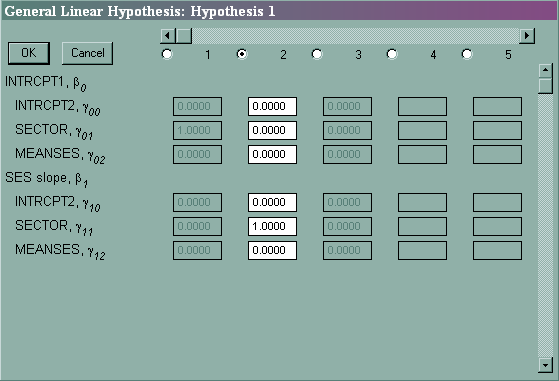
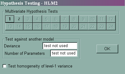
To test the effect of
sector on the intercept and on the ses
slope simultaneously we will choose Hypothesis Testing from the Other
Settings pull-down menu. We will then
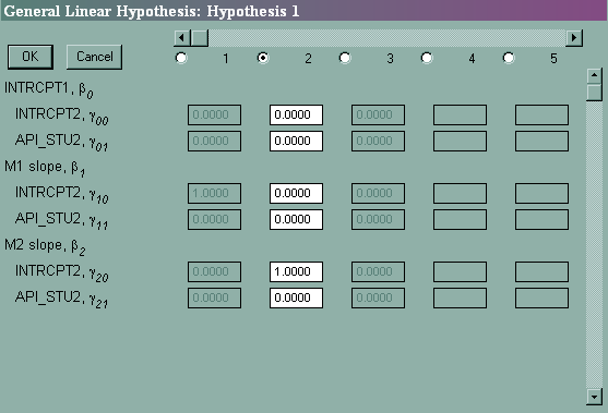
click on the 1 button to specify our first hypothesis (see below).

We then fill out the boxes below to indicate we wish to jointly test
γ₀₁ = 0 and γ₁₁ =
0 .

After specifying your hypothesis test(s) and clicking on OK and OK, rerun the
model and look towards the bottom of the output.

 ----------------------------------------------------------------------------

                Results of General Linear Hypothesis Testing
 -----------------------------------------------------------------------------
                                   Coefficients      Contrast
 -----------------------------------------------------------------------------
 For       INTRCPT1, B0
     INTRCPT2, G00                  12.096006      0.000   0.000
       SECTOR, G01                   1.226384      1.000   0.000
      MEANSES, G02                   5.333056      0.000   0.000
 For      SES slope, B1
     INTRCPT2, G10                   2.937981      0.000   0.000
       SECTOR, G11                  -1.640954      0.000   1.000
      MEANSES, G12                   1.034427      0.000   0.000

Chi-square statistic = 60.596880
Degrees of freedom   = 2
P-value              = 0.000000

4. Multivariate tests of variance-covariance components
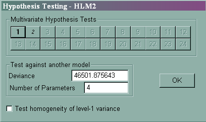
specification

From Model 4 that we ran before, we saw that the p-value for the test of the
variance component of the slope
is not significant. This suggests that we may not want to model the slope as
randomly varying. A simpler model would be that the slope of the variable ses
varies nonrandomly for the level-2 variables sector and meanses. We may
want to compare these two models to decide if the simpler model is comparable
with the previous one.

REML (restricted maximum likelihood) versus FML (full maximum
likelihood)
- REML and FML will usually produce similar results for the level-1
  residual (σ²), but there can be
  noticeable differences for the variance-covariance matrix of the random
  effects.
- REML is the default
  estimation method in HLM.
- If the number of level-2 units is large, then the difference will be
  small.
- If the number of level-2 units is small, then FML variance estimates will
  be smaller than REML, leading to artificially short confidence interval and
  problematic significant tests.
Nested models
- If the fixed effects are the same, and there are fewer random effects in
  the reduced model, then both REML or FML are fine.
- If one model has fewer fixed effects and possibly fewer random
  effects, then use FML to compare models.

Sigma_squared =     36.76611

 Tau
 intrcpt1,B0      2.37524

Tau (as correlations)
 intrcpt1,B0  1.000

 ----------------------------------------------------
  Random level-1 coefficient   Reliability estimate
 ----------------------------------------------------
  intrcpt1, B0                        0.732
 ----------------------------------------------------

The value of the likelihood function at iteration 6 = -2.325148E+004

 Final estimation of fixed effects:
 ----------------------------------------------------------------------------
                                       Standard             Approx.
    Fixed Effect         Coefficient   Error      T-ratio   d.f.     P-value
 ----------------------------------------------------------------------------
 For       intrcpt1, B0
    INTRCPT2, G00          12.096251   0.198643    60.894       157    0.000
      SECTOR, G01           1.224401   0.306117     4.000       157    0.000
     meanses, G02           5.336698   0.368978    14.463       157    0.000
 For      SES slope, B1
    INTRCPT2, G10           2.935860   0.150705    19.481      7179    0.000
      SECTOR, G11          -1.642102   0.233097    -7.045      7179    0.000
     meanses, G12           1.044120   0.291042     3.588      7179    0.001
 ----------------------------------------------------------------------------

 Final estimation of fixed effects
 (with robust standard errors)
 ----------------------------------------------------------------------------
                                       Standard             Approx.
    Fixed Effect         Coefficient   Error      T-ratio   d.f.     P-value
 ----------------------------------------------------------------------------
 For       intrcpt1, B0
    INTRCPT2, G00          12.096251   0.173691    69.642       157    0.000
      SECTOR, G01           1.224401   0.308507     3.969       157    0.000
     meanses, G02           5.336698   0.334617    15.949       157    0.000
 For      SES slope, B1
    INTRCPT2, G10           2.935860   0.147580    19.893      7179    0.000
      SECTOR, G11          -1.642102   0.237223    -6.922      7179    0.000
     meanses, G12           1.044120   0.332897     3.136      7179    0.002
 ----------------------------------------------------------------------------

 Final estimation of variance components:
 -----------------------------------------------------------------------------
 Random Effect           Standard      Variance     df    Chi-square  P-value
                         Deviation     Component
 -----------------------------------------------------------------------------
 intrcpt1,       U0        1.54118       2.37524   157     604.29893    0.000
  level-1,       R         6.06351      36.76611
 -----------------------------------------------------------------------------

 Statistics for current covariance components model
 --------------------------------------------------
 Deviance                       = 46502.952734
 Number of estimated parameters = 2

 Variance-Covariance components test
 -----------------------------------
 Chi-square statistic         =      1.07710
 Number of degrees of freedom =    2
 P-value                      = >.500

Other issues

1. Modeling heterogeneity of level-1 variances

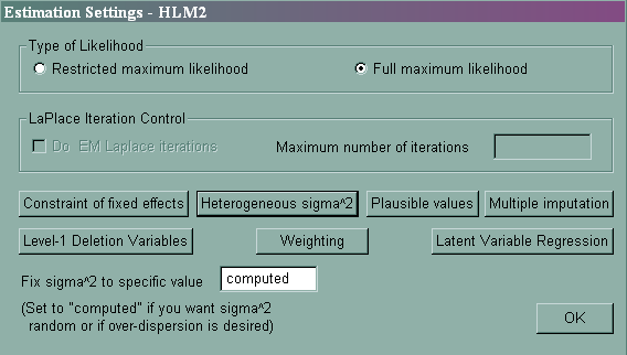
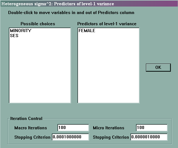
Sometimes, the level-1 variance may be heterogeneous. For example, we may
expect that female students and male students have different variances. Thus,
we want to model the level-1 variance to be a function of the variable female.
From pull-down menu Other Settings, we can choose Estimation
Settings, and then Heterogeneous sigma^2. We then have a choice on which variable(s) to
choose to model the heterogeneity. Here we picked the variable female.
Click on OK and then OK, and rerun the model. From the
output of Summary of Model Fit, we see that the model with heterogeneous
sigma^2 is a better model (with p-value much less than .05).

RESULTS FOR HETEROGENEOUS SIGMA-SQUARED
(macro iteration 4)

 Var(R) = Sigma_squared and
 log(Sigma_squared) = alpha0 + alpha1(FEMALE)


 Model for level-1 variance
 --------------------------------------------------------------------
                                      Standard
    Parameter        Coefficient      Error       Z-ratio   P-value
 --------------------------------------------------------------------
 INTRCPT1    ,alpha0     3.66570      0.024718    148.301     0.000
   FEMALE    ,alpha1    -0.12106      0.033936     -3.567     0.001
 --------------------------------------------------------------------

Summary of Model Fit

 -------------------------------------------------------------------
 Model                                Number of         Deviance
                                      Parameters
 -------------------------------------------------------------------
 1. Homogeneous sigma_squared             10          46494.59261
 2. Heterogeneous sigma_squared           11          46482.09334
 -------------------------------------------------------------------
 Model Comparison                 Chi-square       df    P-value
 -------------------------------------------------------------------
 Model 1 vs Model 2                  12.49926       1     0.001

 Tau
 INTRCPT1,B0      2.29090       0.18183 
      SES,B1      0.18183       0.06325 


Tau (as correlations)
 INTRCPT1,B0  1.000  0.478
      SES,B1  0.478  1.000

 ----------------------------------------------------
  Random level-1 coefficient   Reliability estimate
 ----------------------------------------------------
  INTRCPT1, B0                        0.725
       SES, B1                        0.033
 ----------------------------------------------------

The value of the likelihood function at iteration 2 = -2.324105E+004
The outcome variable is  MATHACH

 Final estimation of fixed effects:
 ----------------------------------------------------------------------------
                                       Standard             Approx.
    Fixed Effect         Coefficient   Error      T-ratio   d.f.     P-value
 ----------------------------------------------------------------------------
 For       INTRCPT1, B0
    INTRCPT2, G00          12.059116   0.196011    61.523       157    0.000
      SECTOR, G01           1.245117   0.301910     4.124       157    0.000
     MEANSES, G02           5.326542   0.363835    14.640       157    0.000
 For      SES slope, B1
    INTRCPT2, G10           2.952729   0.153406    19.248       157    0.000
      SECTOR, G11          -1.644758   0.236725    -6.948       157    0.000
     MEANSES, G12           1.032606   0.295125     3.499       157    0.001
 ----------------------------------------------------------------------------

 The outcome variable is  MATHACH

 Final estimation of fixed effects
 (with robust standard errors)
 ----------------------------------------------------------------------------
                                       Standard             Approx.
    Fixed Effect         Coefficient   Error      T-ratio   d.f.     P-value
 ----------------------------------------------------------------------------
 For       INTRCPT1, B0
    INTRCPT2, G00          12.059116   0.173152    69.645       157    0.000
      SECTOR, G01           1.245117   0.307648     4.047       157    0.000
     MEANSES, G02           5.326542   0.333385    15.977       157    0.000
 For      SES slope, B1
    INTRCPT2, G10           2.952729   0.148115    19.935       157    0.000
      SECTOR, G11          -1.644758   0.239529    -6.867       157    0.000
     MEANSES, G12           1.032606   0.336341     3.070       157    0.003
 ----------------------------------------------------------------------------

 Final estimation of variance components:
 -----------------------------------------------------------------------------
 Random Effect           Standard      Variance     df    Chi-square  P-value
                         Deviation     Component
 -----------------------------------------------------------------------------
 INTRCPT1,       U0        1.51357       2.29090   157     599.75645    0.000
      SES slope, U1        0.25149       0.06325   157     162.54860    0.364
 -----------------------------------------------------------------------------

 Statistics for current covariance components model
 --------------------------------------------------
 Deviance                       = 46482.093344
 Number of estimated parameters = 11

 Model comparison test
 -----------------------------------
 Chi-square statistic         =     19.78230
 Number of degrees of freedom =    7
 P-value                      = 0.006

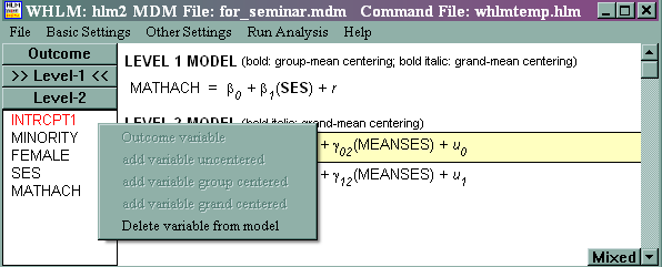
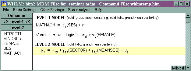
2. Models without a level-1 intercept

Sometimes, we may want to exclude the intercept from our model. For
example, we may have a level-1 categorical variable and we want to include all
the categories of this variable in the model. To accomplish this, we have to exclude
the intercept; otherwise, our model will be over-identified.

3. Constraints of fixed effects

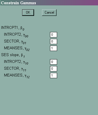
Choose Other Settings then
Estimation
Settings, and then Constraint
of fixed effects. From here, we can constrain, for example, the effect of
γ₀₂to be equal to
γ_12.

Summary of the model specified (in equation format)
 ---------------------------------------------------

Level-1 Model

	Y = B0 + B1*(SES) + R

Level-2 Model
	B0 = G00 + G01*(SECTOR) + G02*(MEANSES) + U0
	B1 = G10 + G11*(SECTOR) + G12*(MEANSES) + U1

	02G = 12G

Iterations stopped due to small change in likelihood function
******* ITERATION 19 *******

 Sigma_squared =     36.75129

 Standard Error of Sigma_squared =      0.62663


 Tau
 INTRCPT1,B0      3.38650      -0.42733 
      SES,B1     -0.42733       0.36901 


 Standard Errors of Tau
 INTRCPT1,B0      0.47559       0.24733 
      SES,B1      0.24733       0.24605 


Tau (as correlations)
 INTRCPT1,B0  1.000 -0.382
      SES,B1 -0.382  1.000

 ----------------------------------------------------
  Random level-1 coefficient   Reliability estimate
 ----------------------------------------------------
  INTRCPT1, B0                        0.795
       SES, B1                        0.162
 ----------------------------------------------------

The value of the likelihood function at iteration 19 = -2.328375E+004
The outcome variable is  MATHACH

 Final estimation of fixed effects:
 ----------------------------------------------------------------------------
                                       Standard             Approx.
    Fixed Effect         Coefficient   Error      T-ratio   d.f.     P-value
 ----------------------------------------------------------------------------
 For       INTRCPT1, B0
    INTRCPT2, G00          11.741607   0.222122    52.861       157    0.000
      SECTOR, G01           2.016592   0.335380     6.013       157    0.000
     MEANSES, G02   *       2.654259   0.237376    11.182       157    0.000
 For      SES slope, B1
    INTRCPT2, G10           3.159636   0.163404    19.336       158    0.000
      SECTOR, G11          -2.096300   0.249567    -8.400       158    0.000
 ----------------------------------------------------------------------------
 The "*" gammas have been constrained.  See the table on the header page.

 The outcome variable is  MATHACH

 Final estimation of fixed effects
 (with robust standard errors)
 ----------------------------------------------------------------------------
                                       Standard             Approx.
    Fixed Effect         Coefficient   Error      T-ratio   d.f.     P-value
 ----------------------------------------------------------------------------
 For       INTRCPT1, B0
    INTRCPT2, G00          11.741607   0.208945    56.195       157    0.000
      SECTOR, G01           2.016592   0.331788     6.078       157    0.000
     MEANSES, G02   *       2.654259   0.253568    10.468       157    0.000
 For      SES slope, B1
    INTRCPT2, G10           3.159636   0.158565    19.926       158    0.000
      SECTOR, G11          -2.096300   0.240992    -8.699       158    0.000
 ----------------------------------------------------------------------------
 The "*" gammas have been constrained.  See the table on the header page.

 Final estimation of variance components:
 -----------------------------------------------------------------------------
 Random Effect           Standard      Variance     df    Chi-square  P-value
                         Deviation     Component
 -----------------------------------------------------------------------------
 INTRCPT1,       U0        1.84024       3.38650   157     787.30255    0.000
      SES slope, U1        0.60746       0.36901   157     192.72983    0.027
  level-1,       R         6.06228      36.75129
 -----------------------------------------------------------------------------

 Statistics for current covariance components model
 --------------------------------------------------
 Deviance                       = 46567.491225
 Number of estimated parameters = 9

4. Level-1 variable as a random effect but not as a fixed effect

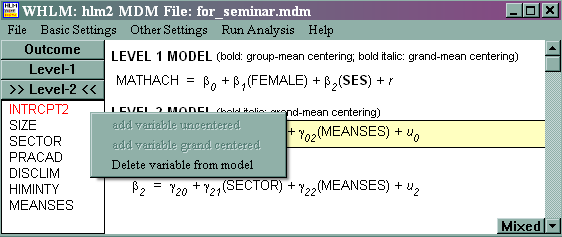
Sometimes, we
may want to model a level-1 variable only as a random effect. For example, the
effect of gender, on average, is not significant, as possibly shown below. In
this case, we may not want to estimate the fixed effect of the variable female.
Instead, we only use the variable female to model the variance.

 Summary of the model specified (in equation format)
 ---------------------------------------------------

Level-1 Model

	Y = B0 + B1*(FEMALE) + B2*(SES) + R

Level-2 Model
	B0 = G00 + G01*(SECTOR) + G02*(meanses) + U0
	B1 = U1
	B2 = G20 + G21*(SECTOR) + G22*(meanses) + U2

Level-1 OLS regressions
 -----------------------

 Level-2 Unit     intrcpt1      FEMALE slope       SES slope  
 ------------------------------------------------------------------------------
        1224     10.94364        -2.06161         2.64284    
        1288     13.01384         1.12946         3.35269    
        1296      8.51189        -1.35628         1.00858    
        1358     11.32162        -0.31470         4.98310    
        1374     10.94983        -2.63062         3.85439    
        1436     19.48721        -4.03507         2.58733    
        1461     17.50503        -1.15047         6.28572

 Sigma_squared =     36.32580

 Standard Error of Sigma_squared =      0.62429

 Tau
 intrcpt1,B0      3.56382      -2.00755       0.33526 
   FEMALE,B1     -2.00755       2.32409      -0.23060 
      SES,B2      0.33526      -0.23060       0.10378

 Standard Errors of Tau
 intrcpt1,B0      0.62400       0.57492       0.26957 
   FEMALE,B1      0.57492       0.72587       0.28483 
      SES,B2      0.26957       0.28483       0.21197

Tau (as correlations)
 intrcpt1,B0  1.000 -0.698  0.551
   FEMALE,B1 -0.698  1.000 -0.470
      SES,B2  0.551 -0.470  1.000

 ----------------------------------------------------
  Random level-1 coefficient   Reliability estimate
 ----------------------------------------------------
  intrcpt1, B0                        0.643
    FEMALE, B1                        0.384
       SES, B2                        0.052
 ----------------------------------------------------

Note: The reliability estimates reported above are based on only 123 of 160
units that had sufficient data for computation.  Fixed effects and variance
components are based on all the data.

The value of the likelihood function at iteration 289 = -2.323661E+004

 Final estimation of fixed effects:
 ----------------------------------------------------------------------------
                                       Standard             Approx.
    Fixed Effect         Coefficient   Error      T-ratio   d.f.     P-value
 ----------------------------------------------------------------------------
 For       intrcpt1, B0
    INTRCPT2, G00          11.933404   0.187148    63.764       157    0.000
      SECTOR, G01           1.180992   0.293859     4.019       157    0.000
     meanses, G02           5.281064   0.353685    14.932       157    0.000
 For      SES slope, B2
    INTRCPT2, G20           2.875972   0.155149    18.537       157    0.000
      SECTOR, G21          -1.615421   0.239356    -6.749       157    0.000
     meanses, G22           1.033760   0.298472     3.464       157    0.001
 ----------------------------------------------------------------------------

 The outcome variable is  mathach

 Final estimation of fixed effects
 (with robust standard errors)
 ----------------------------------------------------------------------------
                                       Standard             Approx.
    Fixed Effect         Coefficient   Error      T-ratio   d.f.     P-value
 ----------------------------------------------------------------------------
 For       intrcpt1, B0
    INTRCPT2, G00          11.933404   0.173443    68.803       157    0.000
      SECTOR, G01           1.180992   0.302841     3.900       157    0.000
     meanses, G02           5.281064   0.330903    15.960       157    0.000
 For      SES slope, B2
    INTRCPT2, G20           2.875972   0.146171    19.675       157    0.000
      SECTOR, G21          -1.615421   0.236022    -6.844       157    0.000
     meanses, G22           1.033760   0.328717     3.145       157    0.002
 ----------------------------------------------------------------------------

 Final estimation of variance components:
 -----------------------------------------------------------------------------
 Random Effect           Standard      Variance     df    Chi-square  P-value
                         Deviation     Component
 -----------------------------------------------------------------------------
 intrcpt1,       U0        1.88781       3.56382   120     326.18770    0.000
   FEMALE slope, U1        1.52450       2.32409   123     187.64867    0.000
      SES slope, U2        0.32214       0.10378   120     122.76674    0.413
  level-1,       R         6.02709      36.32580
 -----------------------------------------------------------------------------

Note: The chi-square statistics reported above are based on only 123 of 160
units that had sufficient data for computation.  Fixed effects and variance
components are based on all the data.

 Statistics for current covariance components model
 --------------------------------------------------
 Deviance                       = 46473.216028
 Number of estimated parameters = 13

5. Testing multi-degree-of-freedom
variables

When using categorical predictor variables that have more than two levels,
you will want to obtain an overall test of the variable. That is, you
will want to know if the categorical variable, taken together, is
statistically significant. As in OLS regression, if the whole
categorical variable (i.e., the multi-degree-of-freedom test) is not
statistically significant, you will not want to interpret any of the single
degree-of-freedom tests of the dummy variables.

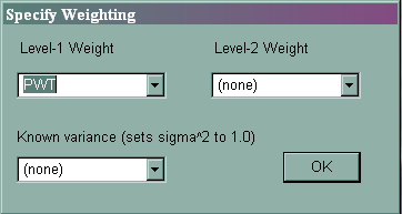
6. Using sampling weights

In the HLM manual, probability weights are called design weights. HLM
can handle weights at both level 1 and level 2. If you
have only a single final sampling weight, specify it as a level 1 variable.
HLM cannot handle other elements that might be present in a survey
data set, such as PSUs, stratification or replicate weights.

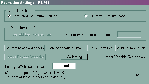
To specify sampling weights at level 1 or level 2, click on Other
Settings, and then Estimation Settings, and then on the
Weighting button.

7. Using multiply imputed data

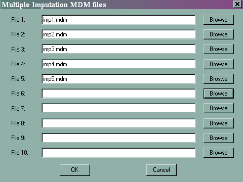
HLM cannot create multiply imputed data sets, but it can analyze them.
HLM can handle only 10 imputed data sets. You must create an
.mdm file for each of the multiply imputed data sets, and you must make
exactly the same variable selections in each of the data sets.

To specify the multiply imputed data sets, click on Other Settings,
and then Estimation Settings, and then on the Multiple imputation
button.

Conclusions

HLM has some very nice features for the analysis of multilevel data.

It has a very intuitive interface for building the model using a
multi-equation format. The mixed button is a nice way to see the mixed
equation (the combination of the multiple equations).
It can create graphs to aid in the interpretation of cross-level
interactions.
While it does not have built in features for producing diagnostic plots,
it easily generates the diagnostic data for use in common statistical
packages.
HLM is very flexible in its ability to read in data. In older
versions of HLM, you needed to create a level 1 and a level 2 data file, but
with the current version, you can both level 1 and level 2 variables in a
single data file. You can easily read in SPSS and Stata data files, as
well data in several other formats.
We have not discussed many of the other types of analysis that HLM can
do, such as three-level models, non-linear models, and cross-classified
models.

References

Multilevel Analysis: An Introduction to Basic and Advanced Multilevel Modeling
by Tom Snijders and Roel Bosker

Introduction
to Multilevel Modeling by Ita Kreft and Jan de Leeuw

Multilevel
Analysis: Techniques and Applications by Joop Hox

Hierarchical Linear Models, Second Edition by Stephen Raudenbush and Anthony
Bryk

HLM 6 – Hierarchical Linear and Nonlinear Modeling by Raudenbush, et al.

Multilevel Analysis for Applied Research: It’s Just Regression! by
Robert Bickel

Power and
Sample Size in Multilevel Modeling by Tom Snijders (in Encyclopedia of
Statistics in Behavioral Science, Everitt and Howell (editors), Vol. 3,
1570-1573)

Outline

Getting data into HLM

The data set

A brief word about sample sizes

Model building

Graphing the results

Model fit

Residual file and analysis of model fit

2. Testing the homogeneity of level-1 variances

3. Multivariate hypothesis tests for fixed effects

4. Multivariate tests of variance-covariance components specification

Other issues

1. Modeling heterogeneity of level-1 variances

2. Models without a level-1 intercept

3. Constraints of fixed effects

4. Level-1 variable as a random effect but not as a fixed effect

5. Testing multi-degree-of-freedom variables

6. Using sampling weights

7. Using multiply imputed data

Conclusions

References

4. Multivariate tests of variance-covariance components
specification

5. Testing multi-degree-of-freedom
variables