
First off, let’s start with what a significant three-way interaction means. It means that
there is a two-way interaction that varies across levels of a third variable. Say, for
example, that a b*c interaction differs across various levels of factor a.
One way of analyzing the three-way interaction is to begin by testing two-way interactions
at each level of a third variable. This process is just a generalization of tests
of simple main effects which can is used for two-way interactions. If you find the
material on this FAQ page to be confusing there is another page which takes a
more conceptual approach that is not stat package specific. That page is located
here.
We will use a small artificial example that has a statistically significant three-way interaction
to illustrate the process.
use https://stats.idre.ucla.edu/stat/stata/faq/threeway, clear

anova y a b c a*b a*c b*c a*b*c

                          Number of obs =      24     R-squared     =  0.9689
                           Root MSE      =  1.1547     Adj R-squared =  0.9403

                  Source |  Partial SS    df       MS           F     Prob > F
              -----------+----------------------------------------------------
                   Model |  497.833333    11  45.2575758      33.94     0.0000
                         |
                       a |         150     1         150     112.50     0.0000
                       b |  .666666667     1  .666666667       0.50     0.4930
                       c |  127.583333     2  63.7916667      47.84     0.0000
                     a*b |  160.166667     1  160.166667     120.13     0.0000
                     a*c |       18.25     2       9.125       6.84     0.0104
                     b*c |  22.5833333     2  11.2916667       8.47     0.0051
                   a*b*c |  18.5833333     2  9.29166667       6.97     0.0098
                         |
                Residual |          16    12  1.33333333
              -----------+----------------------------------------------------
                   Total |  513.833333    23  22.3405797
Next, we need to select a two-way interaction to look at more closely. For the
purposes of this example we will examine the b*c interaction.
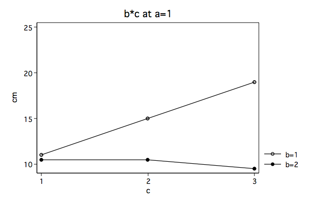
Let’s graph the b*c interaction for each of the two levels of a. We will do this
by computing the cell means for the 12 cells in the design.
egen abc=group(a b c), label
egen cm=mean(y), by(abc)
twoway (connect cm c if a==1 & b==1)(connect cm c if a==1 & b==2), ///
name(at_a_1) xlabel(1(1)3) title("b*c at a=1") ///
ylabel(10(5)25) legend(order(1 "b=1" 2 "b=2"))
 twoway (connect cm c if a==2 & b==1)(connect cm c if a==2 & b==2), ///
name(at_a_2) xlabel(1(1)3) title("b*c at a=2") ///
ylabel(10(5)25) legend(order(1 "b=1" 2 "b=2"))
twoway (connect cm c if a==2 & b==1)(connect cm c if a==2 & b==2), ///
name(at_a_2) xlabel(1(1)3) title("b*c at a=2") ///
ylabel(10(5)25) legend(order(1 "b=1" 2 "b=2"))
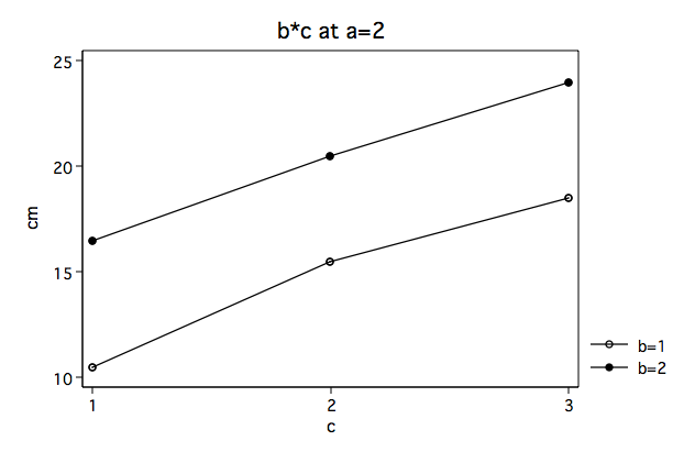
We believe from looking at the two graphs above that the three-way interaction is significant
because there appears to be a “strong” two-way interaction at a = 1 and no interaction at a = 2.
Now, we just have to show it statistically using tests of simple main-effects.
To do that we will make use of some Stata commands
that you will need to paste into your do-file editor.
/* paste commands into do-file */

/* denominator for tests of simple effects - part A */
global mse = e(rss)/e(df_r)
global dfe = e(df_r)

/* numerator for testing 2-way interaction - part B */
global msm = e(ss_3)/e(df_3)
global dfn = e(df_3)
global ftst = $msm/$mse
display "F(" $dfn "," $dfe ") = " $ftst

/* numerator for testing simple main effects - part C */
global msm = e(ss_1)/e(df_1)
global dfn = e(df_1)
global ftst = $msm/$mse
display "F(" $dfn "," $dfe ") = " $ftst
The way we will use these commands is to highlight several lines at a time and run just
the selected lines, which you will see echoed to the output.
We will begin by capturing the residual sums of squares and degrees
of freedom from the full model. For this example, the residual mean-square is the error
term for all of the effects in the model and thus, for all of the tests of simple main-effects.
/* denominator for tests of simple effects - part A */
global mse = e(rss)/e(df_r)
global dfe = e(df_r)

/* run anova model with b & c at a==1 */

anova y b c b*c if a==1

                           Number of obs =      12     R-squared     =  0.9475
                           Root MSE      = 1.11803     Adj R-squared =  0.9038

                  Source |  Partial SS    df       MS           F     Prob > F
              -----------+----------------------------------------------------
                   Model |  135.416667     5  27.0833333      21.67     0.0009
                         |
                       b |  70.0833333     1  70.0833333      56.07     0.0003
                       c |  24.6666667     2  12.3333333       9.87     0.0127
                     b*c |  40.6666667     2  20.3333333      16.27     0.0038
                         |
                Residual |         7.5     6        1.25
              -----------+----------------------------------------------------
                   Total |  142.916667    11  12.9924242

/* numerator for testing 2-way interaction - part B */
global msm = e(ss_3)/e(df_3)
global dfn = e(df_3)
global ftst = $msm/$mse
display "F(" $dfn "," $dfe ") = " $ftst

F(2,12) = 15.25
The F-ratio of 15.25 is the test of the b*c interaction at a = 1.
We will defer the discussion on the critical value for a few
moments while we compute the test of simple main-effects at a = 2.
anova y b c b*c if a==2

                           Number of obs =      12     R-squared     =  0.9615
                           Root MSE      = 1.19024     Adj R-squared =  0.9295

                  Source |  Partial SS    df       MS           F     Prob > F
              -----------+----------------------------------------------------
                   Model |  212.416667     5  42.4833333      29.99     0.0004
                         |
                       b |       90.75     1       90.75      64.06     0.0002
                       c |  121.166667     2  60.5833333      42.76     0.0003
                     b*c |          .5     2         .25       0.18     0.8424
                         |
                Residual |         8.5     6  1.41666667
              -----------+----------------------------------------------------
                   Total |  220.916667    11  20.0833333

/* numerator for testing 2-way interaction - part B */
global msm = e(ss_3)/e(df_3)
global dfn = e(df_3)
global ftst = $msm/$mse
display "F(" $dfn "," $dfe ") = " $ftst

F(2,12) = .1875
Clearly, one F-ratio is much larger than the other but
how can we tell which are statistically significant? There are at least four different methods
of determining the critical value of tests of simple main-effects. There is a method related
to Dunn’s multiple comparisons,
a method attributed to Marascuilo & Levin, a method called the simultaneous test
procedure (very conservative and related to the Scheffé post-hoc test) and a per
family error rate method.
We will demonstrate the per family error rate method but you should look up the other
methods in a good anova book, like Kirk (1995), to decide which approach is best for your
situation. The trick here is that we divide 0.05, our alpha level, by 2 in the
invfprob function because we are doing two tests of simple main-effects.
/* compute critical value */
display "critical value per family error rate = " invfprob($dfn, $dfe, 0.05/2)

critical value per family error rate = 5.0958672
The critical value is approximately 5.1. The first F-ratio of 15.25 is significant while
the second (.1875) is not. In other words, the two-way b*c interaction is significant
at a = 1 but is not significant at a = 2.
In an ideal world we would be done now, but since we live in the “real” world, there is still
more to do because we now need to try to understand the significant two-way interaction at
a = 1; first for b = 1 and then for b = 2.
/* look at differences in c at b==1 when a==1 */

anova y c if b==1 & a==1

                           Number of obs =       6     R-squared     =  0.9143
                           Root MSE      = 1.41421     Adj R-squared =  0.8571

                  Source |  Partial SS    df       MS           F     Prob > F
              -----------+----------------------------------------------------
                   Model |          64     2          32      16.00     0.0251
                         |
                       c |          64     2          32      16.00     0.0251
                         |
                Residual |           6     3           2
              -----------+----------------------------------------------------
                   Total |          70     5          14

/* get infor for c at b==1 & a==1 */
/* numerator for testing simple main effects - part C */
global msm = e(ss_1)/e(df_1)
global dfn = e(df_1)
global ftst = $msm/$mse
display "F(" $dfn "," $dfe ") = " $ftst

F(2,12) = 24

/* look at differences in c at b==2 when a==1 */

anova y c if b==2 & a==1

                           Number of obs =       6     R-squared     =  0.4706
                           Root MSE      = .707107     Adj R-squared =  0.1176

                  Source |  Partial SS    df       MS           F     Prob > F
              -----------+----------------------------------------------------
                   Model |  1.33333333     2  .666666667       1.33     0.3852
                         |
                       c |  1.33333333     2  .666666667       1.33     0.3852
                         |
                Residual |         1.5     3          .5
              -----------+----------------------------------------------------
                   Total |  2.83333333     5  .566666667

/* get infor for c at b==2 & a==1 */
/* numerator for testing simple main effects - part C */
global msm = e(ss_1)/e(df_1)
global dfn = e(df_1)
global ftst = $msm/$mse
display "F(" $dfn "," $dfe ") = " $ftst

F(2,12) = .5

/* compute critical value */
display "critical value per family error rate         = " invfprob($dfn, $dfe, 0.05/2)

critical value per family error rate         = 5.0958672
Only the test of simple main-effects of c at b = 1 was significant. But we’re not done yet,
since there are three levels of c, we don’t know where this significant effect lies. We
need to test the pairwise comparisons among the three means. We will do this using the
tukeyhsd command (search tukeyhsd;
see How can I use the search
command to search for programs?) for our pairwise comparisons. We use an if in the
tukeyhsd command to restrict the pairwise comparisons to b = 1 at a = 1.
/* all pairwise comparisons at a==1 & b==1  */

tukeyhsd c if a==1 & b==1, nu($dfe) mse($mse)

Tukey HSD pairwise comparisons for variable c
studentized range critical value(.05, 3, 12) = 3.772768
uses harmonic mean sample size =    2.000

                                       mean
grp vs grp       group means           dif    HSD-test
-------------------------------------------------------
  1 vs   2    11.0000    15.0000      4.0000   4.8990*
  1 vs   3    11.0000    19.0000      8.0000   9.7980*
  2 vs   3    15.0000    19.0000      4.0000   4.8990*
As shown above, each of the pairwise comparisons among the levels of c at b = 1 are
statistically significant. Hopefully, we now have a much better understanding of the
three-way a*b*c interaction.
The process would have be similar if we had chosen a different two-way interaction back
at the beginning.
Summary of Steps
1) Run full model with three-way interaction.
1a) Capture SS and df residual.
2) Run two-way interaction at each level of third variable.
2a) Capture SS and df for interactions.
2b) Compute F-ratios for tests of interaction at levels of a 3rd variable.
3) Run one-way model at each level of second variable.
3a) Capture SS and df for main effects.
3b) Compute F-ratios for tests of simple main-effects.
4) Run pairwise or other post-hoc comparisons if necessary
Is there some way of computing the various F-ratios for understanding the 3-way interaction
without using global macro variables and doing all of the cutting-and-pasting?
Yes, there is. Is it easier that the method above? No, its just different. Click
on Part 2 to view it.
References
Kirk, Roger E. (1995) Experimental Design: Procedures for the Behavioral Sciences,
Third Edition. Monterey, California: Brooks/Cole Publishing.