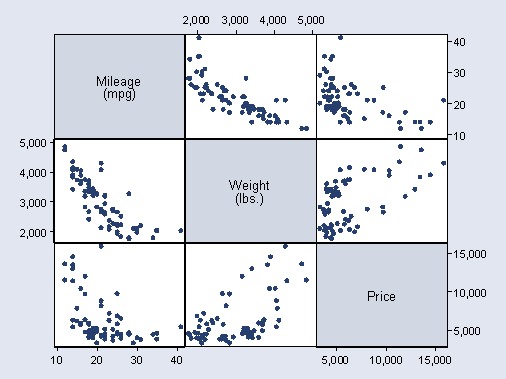
This module will introduce some basic graphs in Stata 12, including histograms, boxplots, scatterplots, and scatterplot matrices.
Let’s use the auto data file for making some graphs.
sysuse auto.dta
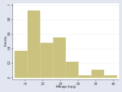
The histogram command can be used to make a simple histogram of mpg
histogram mpg
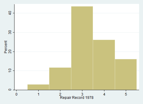
If you are creating a histogram for a categorical variable such as
rep78, you can add the option discrete. As you can see
below, when you specify this option, the midpoint of each bin
labels the respective bar.
hist rep78, percent discrete
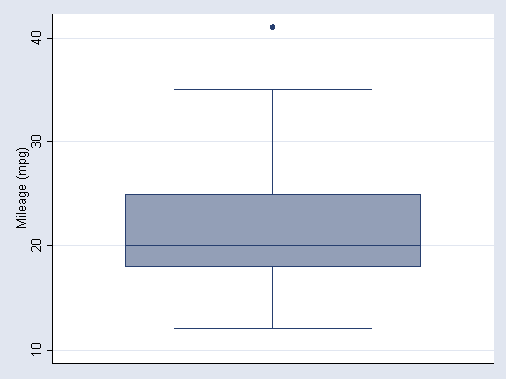
The graph box command can be used to produce a boxplot which can help you examine the distribution of
mpg. If mpg were normally distributed, the line (the median) would be
in the middle of the box (the 25th and 75th percentiles, Q1 and Q3) and the ends
of the whiskers (the upper and lower adjacent values, which are the
most extreme values within Q3+1.5(Q3-Q1) and Q1-1.5*(Q3-Q1),
respectively) would be equidistant from the box. The boxplot for
mpg shows positive skew. The median is pulled to the low end of the box.
graph box mpg
The boxplot can be done separately for foreign
and domestic cars using the by( ) or over( ) option.
graph box mpg, by(foreign)
graph box mpg, over(foreign)
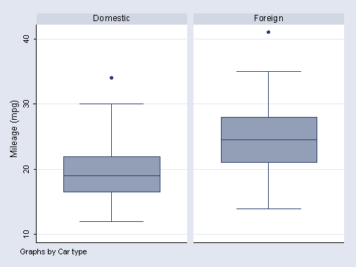
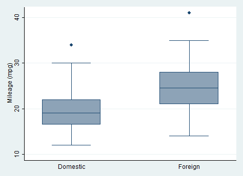
As you can see in the graph above, there are a pair of outliers in the box
plots produced. These can be removed from the box plot using the
noout command in Stata.
graph box mpg, over(foreign) noout
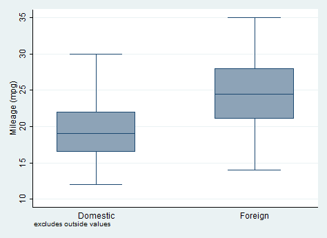
The graph no longer includes the outlying values. Stata also includes a
message at the bottom of the graph noting that outside values were excluded.
Stata can also produce pie charts.
graph pie, over(rep78) plabel(_all name) title("Repair Record 1978")
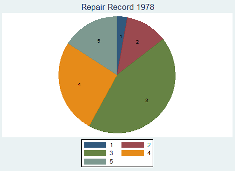
The graph pie command with the over option
creates a pie chart representing the frequency of each group or value of
rep78. The plabel option places the value
labels for rep78 inside each slice of the pie chart.
A two way scatter plot can be used to show the relationship between mpg
and weight. As we would expect, there is a negative relationship between
mpg and weight.
graph twoway scatter mpg weight
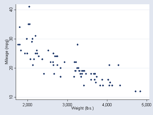
Note that you can save typing like this
twoway scatter mpg weight
We can show the regression line predicting mpg from
weight like this.
twoway lfit mpg weight
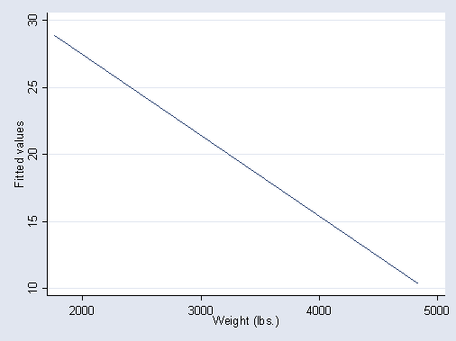
We can combine these graphs like shown below.
twoway (scatter mpg weight) (lfit mpg weight)
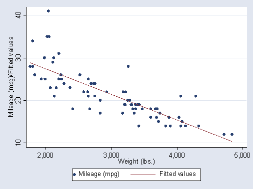
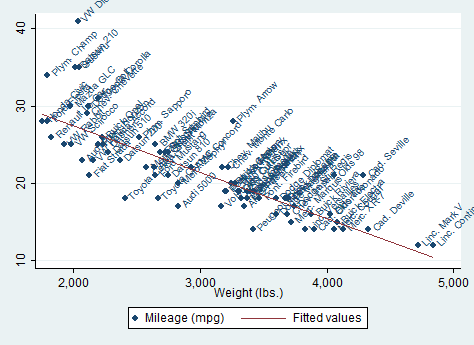
We can add labels to the points labeling them by make as
shown below. Note that mlabel is an option on the scatter command.
twoway (scatter mpg weight, mlabel(make) ) (lfit mpg weight)
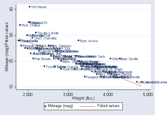
The marker label position can be changed using the mlabangle( )
option.
twoway (scatter mpg weight, mlabel(make) mlabangle(45)) (lfit mpg weight)
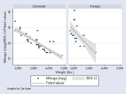
We can combine separate graphs for foreign and domestic cars
as shown below, and we have requested confidence bands around the predicted
values by using lfitci in place of lfit . Note that the by
option is at the end of the command.
twoway (scatter mpg weight) (lfitci mpg weight), by(foreign)
You can request a scatter plot matrix with the graph matrix command. Here we examine the relationships among
mpg, weight
and price.
graph matrix mpg weight price