
This page has been updated to Stata 15.1.
Introduction
The purpose of this seminar is to
help you increase your skills in using logistic regression analysis with Stata. The
seminar does not teach logistic regression, per se, but focuses on how to perform
logistic regression analyses and interpret the results using Stata. It is assumed that you
are familiar with ordinary least squares regression and logistic regression (e.g., have had a class
in logistic regression or have read about logistic regression, see our
Statistics Books for Loan for books you can borrow on
logistic regression). Of course, we will not be discussing all aspects of logistic regression.
This workshop will focus mostly on interpreting the output in these different metrics, rather than on other aspects of the analysis,
such as model building, model diagnostics, receiver-operator curves, sensitivity and specificity.
Community-contributed commands
In addition to the built-in Stata commands we will be demonstrating the use of a
number on community-contributed (AKA user-written) ado-files, in particular, listcoef and fitstat.
To find out more about these programs or to download them type search followed by the
program name in the Stata command window (example: search listcoef). These add-on programs ease
the running and interpretation of ordinal logistic models. You can also download the complete
spostado package by typing the following in the Stata command window:
net from http://www.indiana.edu/~jslsoc/stata/
net install spost9_ado
Although this is a presentation about logistic regression, we are going to start by talking about ordinary
least squares regression (OLS) briefly. Probably the best way to learn about logistic regression is to get a
good foundation in OLS regression, because most things in OLS regression are easy. Also, almost everything
that you know about predictor variables in OLS regression (the variables on the right-hand side) is the same
in logistic regression, expect with respect to certain types of interaction terms, which we will discuss
toward the end of this workshop. The difference between OLS regression and logistic regression is, of course,
the dependent variable: In OLS regression, the dependent (also known as the outcome) variable is continuous,
while in logistic regression it is binary. Please note that when we speak of logistic regression, we really
mean binary logistic regression, as opposed to ordinal logistic regression or multinomial logistic regression.
A binary variable refers to a variable that is coded as 0, 1 or missing; it cannot take on any value other than
those three.
Theoretical treatments of the topic of logistic regression (both binary and ordinal logistic regression) assume
that there is an unobserved, or latent, continuous outcome variable. However, we are able to observe only two states:
0 and 1. In other words, lower values on the latent continuous variable are observed as 0, which higher values
on the latent continuous variable are observed as 1. A point called a threshold (or cutoff) separates the regions
of the latent variable that are observed as 0 and 1. While this explanation helps to make logistic regression seem
a little more like OLS regression, in a practical sense, it isn’t much help.
Consequences of a binary outcome variable
Because we observe 0s and 1s (and perhaps missing values) for the outcome variable in a logistic regression, let’s talk
about the consequences of having such a variable as the outcome variable. First of all, let’s remember that we are modeling the 1s,
which usually means success; 0 usually means failure. There are at least two critical consequences
of having a binary outcome variable. The first is that it requires an increased sample size. We will discuss the reasons
for this later, but for now, keep in mind that logistic regression requires a much larger sample size than OLS regression.
Another important consequence is that we can no longer use an identity link to link our outcome variable with our predictors.
Instead, we will need to use a logit link. This link allows for a linear relationship between the outcome and the predictors;
hence the phrase “linear in the logit.” This means that the coefficients are no longer in the original metric of the variable,
as they are in OLS regression. Instead, the raw coefficients are in the metric of log odds. These log odds (also known as the
log of the odds) can be exponeniated to give an odds ratio. The results can also be converted into predicted probabilities.
So now there are at least three metrics in which the results can be discussed. Each has its own set of pros and cons.
Before continuing on, let’s visit
FAQ: How do I interpret odds ratios in logistic regression? for a quick refresher on the relationship between probability, odds and log odds.
The example data set
For the examples in this workshop, we will use the hsbdemo dataset with the binary response variable honors
(enrolled in an honors English program). Other variables that will be used in example analyses will be read,
which is the score on a reading test; science, which is the score on a science test; socst, which is the score
on a social studies test; female,
which indicates if the student is female (1 = female; 0 = male); and prog, which is the type of
program in which the student is enrolled (1 = general; 2 = academic; 3 = vocational).
Let’s get the dataset into Stata.
use https://stats.idre.ucla.edu/stat/data/hsbdemo, clear
The describe command gives basic information about variables in the dataset.
describe honors read science socst female prog

              storage   display    value
variable name   type    format     label      variable label
---------------------------------------------------------------------------------------------------------------------------------------------------------
honors          float   %19.0g     honlab     honors english
read            float   %9.0g                 reading score
science         float   %9.0g                 science score
socst           float   %9.0g                 social studies score
female          float   %9.0g      fl
prog            float   %9.0g      sel        type of program
In the output above, we see that all of the variables are numeric (storage type is float).
We also see that all three categorical variables (honors, female and prog)
have value labels. These will be shown in the output to make it more meaningful.
The summarize command (which can be shorted to sum) is used to see basic descriptive information on these variables.
summarize honors female read science socst

    Variable |        Obs        Mean    Std. Dev.       Min        Max
-------------+---------------------------------------------------------
      honors |        200        .265    .4424407          0          1
      female |        200        .545    .4992205          0          1
        read |        200       52.23    10.25294         28         76
     science |        200       51.85    9.900891         26         74
       socst |        200      52.405    10.73579         26         71
-------------+---------------------------------------------------------
        prog |        200       2.025    .6904772          1          3
There are several important points to note in the output above. First, all of the variables have 200 observations, so we will
not have issues with missing data. Secondly, as expected, the mean of honors is rather low because relatively few students
are admitted to honors English. The mean of female is approximately 0.5, which means that approximately half of the
students in this sample are female. The mean of the continuous variables read, science and socst are similar,
as are the ranges for these variables.
Below are one-way tabulations of the three categorical variables. We can use the numlabel, add command to add the numeric value
of each category to the descriptive label. That way, you can see both the numeric value and the descriptive label in the output.
numlabel, add
tab1 honors female prog

-> tabulation of honors

 honors english |      Freq.     Percent        Cum.
----------------+-----------------------------------
0. not enrolled |        147       73.50       73.50
    1. enrolled |         53       26.50      100.00
----------------+-----------------------------------
          Total |        200      100.00

-> tabulation of female

     female |      Freq.     Percent        Cum.
------------+-----------------------------------
    0. male |         91       45.50       45.50
  1. female |        109       54.50      100.00
------------+-----------------------------------
      Total |        200      100.00

-> tabulation of prog

    type of |
    program |      Freq.     Percent        Cum.
------------+-----------------------------------
 1. general |         45       22.50       22.50
2. academic |        105       52.50       75.00
3. vocation |         50       25.00      100.00
------------+-----------------------------------
      Total |        200      100.00
In our logistic regression model, the binary variable honors will be the outcome variable. It is important
that the outcome variable in a binary logistic regression is coded as 0 and 1 (and missing, if there are missing
values on that variable). In most statistical software programs, values greater than 1 will be considered to be 1,
which may not be what you intend. (In such situations, an ordered logistic regression or a multinomial logistic
regression may be more appropriate. Those types of logistic regression will not be covered in this presentation.)
Remember that we will be modeling the 1s, which means the 1s category will be compared to the 0 category.
Another point to mention is distribution of the variable honors. It is distributed approximately 75 5 and 25%. This is not bad. In general, logistic
regression will have the most power statistically when the outcome is distributed 50/50. Power will decrease as the distribution becomes more lopsided.
A quick note about running logistic regression in Stata. The output from the logit
command will be in units of log odds. The or option can be added to get odds ratios. Alternatively, the
logistic command can be used; the default output for the logistic command is odds ratios.
Models without interactions
A null model
Let’s start with a null model, which is a model without any predictor variables. In an equation, we are modeling
logit(p)= ß0
logit honors

Iteration 0:   log likelihood = -115.64441
Iteration 1:   log likelihood = -115.64441

Logistic regression                             Number of obs     =        200
                                                LR chi2(0)        =      -0.00
                                                Prob > chi2       =          .
Log likelihood = -115.64441                     Pseudo R2         =    -0.0000

------------------------------------------------------------------------------
      honors |      Coef.   Std. Err.      z    P>|z|     [95% Conf. Interval]
-------------+----------------------------------------------------------------
       _cons |  -1.020141   .1602206    -6.37   0.000    -1.334167    -.706114
------------------------------------------------------------------------------
This means log(p/(1-p)) = -1.020141. What is p here? It turns out that p is the overall probability of being in honors
English (honors = 1). Let’s take a look at the frequency table for honors.
tab honors

 honors english |      Freq.     Percent        Cum.
----------------+-----------------------------------
0. not enrolled |        147       73.50       73.50
    1. enrolled |         53       26.50      100.00
----------------+-----------------------------------
          Total |        200      100.00
So p = 53/200 = .265. The odds are .265/(1-.265) = .3605442 and the log of the odds (logit) is log(.3605442) = -1.020141.
In other words, the intercept from the model with no predictor variables is the estimated log odds of being in honors
English for the whole population of interest. We can get this value from Stata using the logistic command (or logit, or).
logistic honors

Logistic regression                             Number of obs     =        200
                                                LR chi2(0)        =      -0.00
                                                Prob > chi2       =          .
Log likelihood = -115.64441                     Pseudo R2         =    -0.0000

------------------------------------------------------------------------------
      honors |       Odds   Std. Err.      z    P>|z|     [95% Conf. Interval]
-------------+----------------------------------------------------------------
       _cons |   .3605442   .0577666    -6.37   0.000     .2633774    .4935584
------------------------------------------------------------------------------
We can calculate the odds by hand based on the values from the frequency values in the table from above.
display 53/147
.36054422
We can also transform the log of the odds back to a probability:
p = exp(-1.020141)/(1+exp(-1.020141)) = .26499994, if we like. We can have Stata calculate this value for us by using the
margins command.
margins
Warning: prediction constant over observations.

Predictive margins                              Number of obs     =        200
Model VCE    : OIM

Expression   : Pr(honors), predict()

------------------------------------------------------------------------------
             |            Delta-method
             |     Margin   Std. Err.      z    P>|z|     [95% Conf. Interval]
-------------+----------------------------------------------------------------
       _cons |       .265    .031207     8.49   0.000     .2038355    .3261645
------------------------------------------------------------------------------
One binary predictor
Let’s add one binary predictor, female. We will use the logit, or command to get output in terms of odds ratios.
We will then see how the odds ratio can be calculated by hand.
logit(p) = ß0 + ß1*female
logit honors female, or

Iteration 0:   log likelihood = -115.64441
Iteration 1:   log likelihood = -113.68907
Iteration 2:   log likelihood = -113.67691
Iteration 3:   log likelihood =  -113.6769

Logistic regression                             Number of obs     =        200
                                                LR chi2(1)        =       3.94
                                                Prob > chi2       =     0.0473
Log likelihood =  -113.6769                     Pseudo R2         =     0.0170

------------------------------------------------------------------------------
      honors | Odds Ratio   Std. Err.      z    P>|z|     [95% Conf. Interval]
-------------+----------------------------------------------------------------
      female |   1.918168   .6400451     1.95   0.051     .9973827    3.689024
       _cons |   .2465754   .0648892    -5.32   0.000     .1472129    .4130033
------------------------------------------------------------------------------
Note: _cons estimates baseline odds.
In our dataset, what are the odds of a male being in honors English and what are the odds of a female being in the honors English?
We can manually calculate these odds from the table: for males, the odds of being in the honors class are (18/91)/(73/91) = .24657534;
and for females, the odds of being in the honors class are (35/109)/(74/109) = .47297297. The ratio of the odds for female to the odds
for male is (73/18)/(74/35) = (73*35)/(74*18) = 1.9181682. So the odds for males are 18 to 73, the odds for females are 35 to 74, and the odds
for female are about 92% higher than the odds for males.
logit honors female

Iteration 0:   log likelihood = -115.64441
Iteration 1:   log likelihood = -113.68907
Iteration 2:   log likelihood = -113.67691
Iteration 3:   log likelihood =  -113.6769

Logistic regression                             Number of obs     =        200
                                                LR chi2(1)        =       3.94
                                                Prob > chi2       =     0.0473
Log likelihood =  -113.6769                     Pseudo R2         =     0.0170

------------------------------------------------------------------------------
      honors |      Coef.   Std. Err.      z    P>|z|     [95% Conf. Interval]
-------------+----------------------------------------------------------------
      female |   .6513706   .3336752     1.95   0.051    -.0026207    1.305362
       _cons |  -1.400088   .2631619    -5.32   0.000    -1.915875   -.8842998
------------------------------------------------------------------------------
Now we can relate the odds for males and females and the output from the logistic regression. The intercept of -1.40 is the log odds
for males because male is the reference group (female = 0). Using the odds we calculated above for males, we can confirm this: log(.2465754) = -1.400088.
The coefficient for female is the log of odds ratio between the female group and male group: log(1.918168) = .65137056. So we can get the odds ratio
by exponentiating the coefficient for female.
The odds ratio for the variable female is 1.918168. Let’s see how we could calculate this number
from the crosstabulation of honors and female.
We can use the formula: (a/c)/(b/d) or, equivalently, a*d/b*c.
tab honors female, chi2

      honors |        female
     english |      male     female |     Total
-------------+----------------------+----------
not enrolled |        73         74 |       147
    enrolled |        18         35 |        53
-------------+----------------------+----------
       Total |        91        109 |       200

          Pearson chi2(1) =   3.8710   Pr = 0.049
We have (male-not enrolled/male-enrolled)/(female-not enrolled/female-enrolled).
display (73/18)/(74/35)
1.9181682
Alternatively, we could use (male-not enrolled*female-enrolled)/(female-not enrolled*male-enrolled).
display (73*35)/(74*18)
1.9181682
Looking back at the crosstabulation above, notice that all of the cells have a reasonable number of observations in them. It is good practice to do a crosstab
of the outcome variable and all of the categorical predictors before running a logistic regression to check for empty or sparse cells. The possible consequences of
having empty cells or cells with very few observations include the model not converging or the confidence intervals being very wide.
Let’s review the interpretation of both the odds ratio and the raw coefficient of this model. We will rerun each model for clarity.
logit honors female, or

Iteration 0:   log likelihood = -115.64441
Iteration 1:   log likelihood = -113.68907
Iteration 2:   log likelihood = -113.67691
Iteration 3:   log likelihood =  -113.6769

Logistic regression                             Number of obs     =        200
                                                LR chi2(1)        =       3.94
                                                Prob > chi2       =     0.0473
Log likelihood =  -113.6769                     Pseudo R2         =     0.0170

------------------------------------------------------------------------------
      honors | Odds Ratio   Std. Err.      z    P>|z|     [95% Conf. Interval]
-------------+----------------------------------------------------------------
      female |   1.918168   .6400451     1.95   0.051     .9973827    3.689024
       _cons |   .2465754   .0648892    -5.32   0.000     .1472129    .4130033
------------------------------------------------------------------------------
Note: _cons estimates baseline odds.
The general interpretation of an exponetiated logistic regression coefficient is this (Long and Freese, 2014, page 229):
“For a unit change in xk, the odds are expected to change by a factor of exp(bk), holding all other variables constant.”
The interpretation of this odds ratio is that, for a one-unit increase in female (in other words,
going from male to female), the odds of being enrolled in honors English increases by a factor of 1.9, holding all other variables constant.
One other thing to note about reporting odds ratios. When reporting odds ratios, you usually report the associated 95% confidence interval, rather than the
standard error. This is because the odds ratio is a nonlinear transformation of the logit coefficient, so the confidence interval is asymmetric.
logit honors female

Iteration 0:   log likelihood = -115.64441
Iteration 1:   log likelihood = -113.68907
Iteration 2:   log likelihood = -113.67691
Iteration 3:   log likelihood =  -113.6769

Logistic regression                             Number of obs     =        200
                                                LR chi2(1)        =       3.94
                                                Prob > chi2       =     0.0473
Log likelihood =  -113.6769                     Pseudo R2         =     0.0170

------------------------------------------------------------------------------
      honors |      Coef.   Std. Err.      z    P>|z|     [95% Conf. Interval]
-------------+----------------------------------------------------------------
      female |   .6513706   .3336752     1.95   0.051    -.0026207    1.305362
       _cons |  -1.400088   .2631619    -5.32   0.000    -1.915875   -.8842998
------------------------------------------------------------------------------
The general interpretation of a logistic regression coefficient is this (Long and Freese, 2014, page 228): “For a unit change
in xk, we expect the log of the odds of the outcome to change bk units, holding all other variables constant.”
For this example, we would say that for a one-unit increase in female (in other words, going from male to female), the expected log of the odds
of being in honors English increases by 0.65, holding all other variables constant.
There are a couple of other points to discuss regarding the output from our first logistic regression.
The model is given again below for ease of reference.
logit honors female, or

Iteration 0:   log likelihood = -115.64441
Iteration 1:   log likelihood = -113.68907
Iteration 2:   log likelihood = -113.67691
Iteration 3:   log likelihood =  -113.6769

Logistic regression                             Number of obs     =        200
                                                LR chi2(1)        =       3.94
                                                Prob > chi2       =     0.0473
Log likelihood =  -113.6769                     Pseudo R2         =     0.0170

------------------------------------------------------------------------------
      honors | Odds Ratio   Std. Err.      z    P>|z|     [95% Conf. Interval]
-------------+----------------------------------------------------------------
      female |   1.918168   .6400451     1.95   0.051     .9973827    3.689024
       _cons |   .2465754   .0648892    -5.32   0.000     .1472129    .4130033
------------------------------------------------------------------------------
Note: _cons estimates baseline odds.
First, while using the nolog option will shorten your output (by no displaying the iteration log)
and is commonly used in examples, in real research, that part of the output can be an important source
of information if there is a problem with your model. For example, sometimes logistic regression models
don’t converge. If you don’t show the iteration log, you can’t see that problem.
Second, remember that logistic regression is a maximum likelihood procedure (you can see the log likelihood
in the output). All maximum likelihood procedures require relatively large sample sizes because of the
assumptions that they make. Also, the outcome variable in a logistic regression is binary, which means that
it necessarily contains less information than other types of outcomes, such as a continuous outcome. Long
(1997, page 54) states: “It is risky to use ML with samples smaller than 100, while sample over 500 seem adequate.
These values should be raised depending on characteristics of the model and data.”
Third, let’s talk about the pseudo R-squared. The emphasis is the on the term “pseudo”. A pseudo R-squared is not
comparable to the R-squared that you would get from an ordinary least squares regression. This means that you cannot
interpret it as the percentage of variance in the outcome that is accounted for by the model. Rather, this value is
good for comparing the relative fit of two models, but it says nothing about the absolute fit of the models. Stata
reports McFadden’s pseudo R-squared, but there are several others.
Please see FAQ: What are pseudo R-squareds? for more information.
Fourth, notice that the p-value for the overall model is statistically significant, while the p-value for the variable
female is not (p = 0.051). Why are they not the same? After all, the variable female is the only predictor
in the model. The answer is that the test of the overall model is a likelihood ratio chi-square, while the test of the
coefficient is a Wald chi-square. Asymptotically, these two tests are equivalent. However, with smaller sample sizes,
a difference can be seen. It is rare that one test would be statistically significant while the other is not. However,
notice that the likelihood ratio test is “just barely” statistically significant, while the Wald chi-square is “just
barely” not statistically significant. So, in reality, the results are not that different. Results like these should be
interpreted with caution. Notice also that the p-value for the chi-square analysis above has a p-value of 0.049. This is a Pearson chi-square,
which is also asymptotically equal to the other types of chi-square. As with the other p-values, this p-value is very close to the 0.05 cut off.
Interpreting negative coefficients
Let’s pause for a moment to make sure that we understand how to interpret a logistic regression coefficient that is negative. Let’s suppose that the
logistic regression coefficient is -2. A negative coefficient means
that the predictor variable has a negative relationship with the outcome variable: as one goes up, the other goes down. Using the standard interpretation,
we could say that for a one-unit increase in the predictor, the log of the odds is expected to decrease by 2, holding all other variables constant. Now what about
in the odds ratio metric? First,
exp(-2) = .13533528
Using the standard interpretation, we would say that the for a one-unit increase in the predictor, the odds are expected to decreases by a factor of .14, holding
all other variables constant.
This doesn’t seem like a big change, but remember that odds ratios are multiplicative coefficients. Long and Freese (2014) write on page 223:
“When interpreting odds ratios, remember that they are multiplicative. This means that 1 indicates no effect, positive effects are greater than 1, and negative
effects are between 0 and 1. Magnitudes of positive and negative effects should be compared by taking the inverse of the negative effect, or vice versa. For example, an
odds ratio of 2 has the same magnitude as an odds ratio of 0.5 = 1/2. Thus an odds ratio of 0.1 = 1/10 is much “larger” than the odds ratio of 2 = 1/0.5.
Another consequence of the multiplicative scale is that to determine the effect on the odds of the event not occurring, you simply take the inverse of the effect on the
odds of the event occurring.”
Let’s look at a table of coefficients and odds ratios of equivalent magnitudes. It shows the effect of compressing all of the negative coefficients into odds ratios that range from 0 to 1.
Coefficient  Positive    Negative
0            1           1
1            2.7182818   .36787944
1.5          4.4816891   .22313016
2            7.3890561   .13533528
2.5          12.182494   .082085
3            20.085537   .04978707
One multi-categorical predictor
Now let’s use a different categorical predictor variable. The variable prog has three levels; the lowest-numbered
category will be used as the reference group by default. In this dataset, that level is called “general”.
We will start with a crosstab.
tab honors prog

                |         type of program
 honors english | 1. genera  2. academ  3. vocati |     Total
----------------+---------------------------------+----------
0. not enrolled |        38         65         44 |       147
    1. enrolled |         7         40          6 |        53
----------------+---------------------------------+----------
          Total |        45        105         50 |       200
While there are large differences in the number of observations in each cell, the frequencies are probably large enough to avoid any real problems.
logit honors i.prog

Iteration 0:   log likelihood = -115.64441
Iteration 1:   log likelihood =  -107.7993
Iteration 2:   log likelihood = -107.57279
Iteration 3:   log likelihood =  -107.5719
Iteration 4:   log likelihood =  -107.5719

Logistic regression                             Number of obs     =        200
                                                LR chi2(2)        =      16.15
                                                Prob > chi2       =     0.0003
Log likelihood =  -107.5719                     Pseudo R2         =     0.0698

------------------------------------------------------------------------------
      honors |      Coef.   Std. Err.      z    P>|z|     [95% Conf. Interval]
-------------+----------------------------------------------------------------
        prog |
   academic  |   1.206168   .4577746     2.63   0.008     .3089465     2.10339
   vocation  |  -.3007541   .5988045    -0.50   0.615    -1.474389    .8728812
             |
       _cons |  -1.691676   .4113064    -4.11   0.000    -2.497822   -.8855303
------------------------------------------------------------------------------
In the output above, we can see that the overall model is statistically significant (p = 0.0003). In the output
table, we can see that the “academic” level is statistically significantly different from “general”, while the “vocation” level is not.
We can use the contrast command to get the multi-degree-of-freedom test of the variable prog. This is a Wald chi-square test.
contrast prog

Contrasts of marginal linear predictions

Margins      : asbalanced

------------------------------------------------
             |         df        chi2     P>chi2
-------------+----------------------------------
        prog |          2       14.26     0.0008
------------------------------------------------
Again we see that the p-value for the overall model does not match that given for the variable prog, even though
prog is the only predictor in the model. However, both tests lead to the same conclusion: the variable prog
is a statistically significant predictor of honors. When writing about these results, you would say that the variable
prog was a statistically significant predictor of the outcome variable honors, citing either the LR chi-square
test or the Wald chi-square test, and that there was a statistically significant difference between the “academic” and “general” levels.
While that is important information to convey to your audience, you might want to include something a little more descriptive
and potentially more practical. For this purpose, you can use the margins command. Used after a logistic regression,
the margins command gives the average predicted probabilities of each group.
margins prog

Adjusted predictions                            Number of obs     =        200
Model VCE    : OIM

Expression   : Pr(honors), predict()

------------------------------------------------------------------------------
             |            Delta-method
             |     Margin   Std. Err.      z    P>|z|     [95% Conf. Interval]
-------------+----------------------------------------------------------------
        prog |
    general  |   .1555556   .0540284     2.88   0.004     .0496619    .2614493
   academic  |   .3809524   .0473917     8.04   0.000     .2880663    .4738385
   vocation  |        .12   .0459565     2.61   0.009     .0299269    .2100731
------------------------------------------------------------------------------
The average predicted probability for the reference level, “general”, is 0.156. This isn’t too different from the average
predicted probability for the “vocation” level, 0.12. However, the “academic” level has an average predicted probability of
0.38. This is very different from the average predicted probability of 0.156 of the reference level “general” and explains
why that comparison is statistically significant. The term “average predicted probability” means that, for example, if
everyone in the dataset was treated as if he/she was in the “general” level, then the predicted probability would be 0.156.
It is important to remember that the predicted probabilities will change as the model changes. For example, if another
predictor is added to the model, the predicted probabilities for each level of prog will change. When other
predictor variables are included in the model, it is important to set those to informative values (or at least note the value),
because predicted probabilities are a non-linear metric, which means that the value of the predicted probability depends on the
level at which other variables in the model are held. We will see an example of this a little later.
Also, the p-values in this table test the null hypothesis that the predicted probability is 0. For many purposes, this is an
uninteresting test, and so this is ignored.
Let’s return to our model to review the interpretation of the output.
logit honors i.prog

Iteration 0:   log likelihood = -115.64441
Iteration 1:   log likelihood =  -107.7993
Iteration 2:   log likelihood = -107.57279
Iteration 3:   log likelihood =  -107.5719
Iteration 4:   log likelihood =  -107.5719

Logistic regression                             Number of obs     =        200
                                                LR chi2(2)        =      16.15
                                                Prob > chi2       =     0.0003
Log likelihood =  -107.5719                     Pseudo R2         =     0.0698

------------------------------------------------------------------------------
      honors |      Coef.   Std. Err.      z    P>|z|     [95% Conf. Interval]
-------------+----------------------------------------------------------------
        prog |
2. academic  |   1.206168   .4577746     2.63   0.008     .3089465     2.10339
3. vocation  |  -.3007541   .5988045    -0.50   0.615    -1.474389    .8728812
             |
       _cons |  -1.691676   .4113064    -4.11   0.000    -2.497822   -.8855303
------------------------------------------------------------------------------

logit honors i.prog, or

Iteration 0:   log likelihood = -115.64441
Iteration 1:   log likelihood =  -107.7993
Iteration 2:   log likelihood = -107.57279
Iteration 3:   log likelihood =  -107.5719
Iteration 4:   log likelihood =  -107.5719

Logistic regression                             Number of obs     =        200
                                                LR chi2(2)        =      16.15
                                                Prob > chi2       =     0.0003
Log likelihood =  -107.5719                     Pseudo R2         =     0.0698

------------------------------------------------------------------------------
      honors | Odds Ratio   Std. Err.      z    P>|z|     [95% Conf. Interval]
-------------+----------------------------------------------------------------
        prog |
2. academic  |   3.340659   1.529269     2.63   0.008      1.36199    8.193899
3. vocation  |   .7402597   .4432709    -0.50   0.615     .2289184    2.393798
             |
       _cons |   .1842105    .075767    -4.11   0.000      .082264    .4124954
------------------------------------------------------------------------------
Note: _cons estimates baseline odds.
Assuming that the 2 df test of prog is statistically significant (it is), we can interpret the coefficient for “academic” as:
Being in the academic program compared to the general program, the expected log of the odds increases by 1.2, holding all other variables constant.
Alternatively, we could say that being in the academic program compared to the general program increases the odds of being in honors English by
a factor of 3.34, holding all other variables in the model constant.
Logistic regression models with many categorical predictors
We are not going to run any models with multiple categorical predictor variables, but let’s pretend that we were. Let’s say that we
were going to include both female and prog in our model. There are at least two commands that can be used to do this three-way crosstab.
One is the built-in (AKA native to Stata) command table. The other is a community-contributed (AKA user-written) command tablist.
Of course, both give the same information; the difference is in the way the information is presented.
table honors female prog

--------------------------------------------------------------------------------------
                |                      type of program and female
                | ---- 1. general ----    ---- 2. academic ---    ---- 3. vocation ---
 honors english |   0. male  1. female      0. male  1. female      0. male  1. female
----------------+---------------------------------------------------------------------
0. not enrolled |        19         19           32         33           22         22
    1. enrolled |         2          5           15         25            1          5
--------------------------------------------------------------------------------------

tablist honors female prog

  +---------------------------------------------------------------------------------+
  |          honors      female          prog   _Freq_   _Perc_   _CFreq_   _CPerc_ |
  |---------------------------------------------------------------------------------|
  | 0. not enrolled   1. female   2. academic       33    16.50        33     16.50 |
  | 0. not enrolled     0. male   2. academic       32    16.00        65     32.50 |
  |     1. enrolled   1. female   2. academic       25    12.50        90     45.00 |
  | 0. not enrolled   1. female   3. vocation       22    11.00       112     56.00 |
  | 0. not enrolled     0. male   3. vocation       22    11.00       134     67.00 |
  |---------------------------------------------------------------------------------|
  | 0. not enrolled     0. male    1. general       19     9.50       153     76.50 |
  | 0. not enrolled   1. female    1. general       19     9.50       172     86.00 |
  |     1. enrolled     0. male   2. academic       15     7.50       187     93.50 |
  |     1. enrolled   1. female   3. vocation        5     2.50       192     96.00 |
  |     1. enrolled   1. female    1. general        5     2.50       197     98.50 |
  |---------------------------------------------------------------------------------|
  |     1. enrolled     0. male    1. general        2     1.00       199     99.50 |
  |     1. enrolled     0. male   3. vocation        1     0.50       200    100.00 |
  +---------------------------------------------------------------------------------+
Both of these commands can be modified to include more categorical variables. For example, let’s add
ses and schyp.
table honors female prog, by(ses schtyp)

--------------------------------------------------------------------------------------
ses, type of    |                      type of program and female
school and      | ---- 1. general ----    ---- 2. academic ---    ---- 3. vocation ---
honors english  |   0. male  1. female      0. male  1. female      0. male  1. female
----------------+---------------------------------------------------------------------
1. low          |
1. public       |
0. not enrolled |         7          5            3          9            4          6
    1. enrolled |                    2            1          6                       2
----------------+---------------------------------------------------------------------
1. low          |
2. private      |
0. not enrolled |                    2
    1. enrolled |
----------------+---------------------------------------------------------------------
2. middle       |
1. public       |
0. not enrolled |         9          6            9         12           13         13
    1. enrolled |                    2            5          4            1          2
----------------+---------------------------------------------------------------------
2. middle       |
2. private      |
0. not enrolled |         1          2            8          4            1          1
    1. enrolled |                                            2
----------------+---------------------------------------------------------------------
3. high         |
1. public       |
0. not enrolled |         2          3            9          7            4          2
    1. enrolled |         2          1            8          8                       1
----------------+---------------------------------------------------------------------
3. high         |
2. private      |
0. not enrolled |                    1            3          1
    1. enrolled |                                 1          5
--------------------------------------------------------------------------------------

tablist honors female prog ses schtyp

  +----------------------------------------------------------------------------------------------------------+
  |          honors      female          prog         ses       schtyp   _Freq_   _Perc_   _CFreq_   _CPerc_ |
  |----------------------------------------------------------------------------------------------------------|
  | 0. not enrolled     0. male   3. vocation   2. middle    1. public       13     6.50        13      6.50 |
  | 0. not enrolled   1. female   3. vocation   2. middle    1. public       13     6.50        26     13.00 |
  | 0. not enrolled   1. female   2. academic   2. middle    1. public       12     6.00        38     19.00 |
  | 0. not enrolled     0. male   2. academic   2. middle    1. public        9     4.50        47     23.50 |
  | 0. not enrolled     0. male    1. general   2. middle    1. public        9     4.50        56     28.00 |
  |----------------------------------------------------------------------------------------------------------|
  | 0. not enrolled     0. male   2. academic     3. high    1. public        9     4.50        65     32.50 |
  | 0. not enrolled   1. female   2. academic      1. low    1. public        9     4.50        74     37.00 |
  |     1. enrolled   1. female   2. academic     3. high    1. public        8     4.00        82     41.00 |
  |     1. enrolled     0. male   2. academic     3. high    1. public        8     4.00        90     45.00 |
  | 0. not enrolled     0. male   2. academic   2. middle   2. private        8     4.00        98     49.00 |
  |----------------------------------------------------------------------------------------------------------|
  | 0. not enrolled   1. female   2. academic     3. high    1. public        7     3.50       105     52.50 |
  | 0. not enrolled     0. male    1. general      1. low    1. public        7     3.50       112     56.00 |
  |     1. enrolled   1. female   2. academic      1. low    1. public        6     3.00       118     59.00 |
  | 0. not enrolled   1. female    1. general   2. middle    1. public        6     3.00       124     62.00 |
  | 0. not enrolled   1. female   3. vocation      1. low    1. public        6     3.00       130     65.00 |
  |----------------------------------------------------------------------------------------------------------|
  | 0. not enrolled   1. female    1. general      1. low    1. public        5     2.50       135     67.50 |
  |     1. enrolled   1. female   2. academic     3. high   2. private        5     2.50       140     70.00 |
  |     1. enrolled     0. male   2. academic   2. middle    1. public        5     2.50       145     72.50 |
  | 0. not enrolled   1. female   2. academic   2. middle   2. private        4     2.00       149     74.50 |
  |     1. enrolled   1. female   2. academic   2. middle    1. public        4     2.00       153     76.50 |
  |----------------------------------------------------------------------------------------------------------|
  | 0. not enrolled     0. male   3. vocation      1. low    1. public        4     2.00       157     78.50 |
  | 0. not enrolled     0. male   3. vocation     3. high    1. public        4     2.00       161     80.50 |
  | 0. not enrolled   1. female    1. general     3. high    1. public        3     1.50       164     82.00 |
  | 0. not enrolled     0. male   2. academic     3. high   2. private        3     1.50       167     83.50 |
  | 0. not enrolled     0. male   2. academic      1. low    1. public        3     1.50       170     85.00 |
  |----------------------------------------------------------------------------------------------------------|
  |     1. enrolled   1. female    1. general      1. low    1. public        2     1.00       172     86.00 |
  | 0. not enrolled   1. female   3. vocation     3. high    1. public        2     1.00       174     87.00 |
  | 0. not enrolled     0. male    1. general     3. high    1. public        2     1.00       176     88.00 |
  | 0. not enrolled   1. female    1. general   2. middle   2. private        2     1.00       178     89.00 |
  | 0. not enrolled   1. female    1. general      1. low   2. private        2     1.00       180     90.00 |
  |----------------------------------------------------------------------------------------------------------|
  |     1. enrolled   1. female   2. academic   2. middle   2. private        2     1.00       182     91.00 |
  |     1. enrolled   1. female   3. vocation   2. middle    1. public        2     1.00       184     92.00 |
  |     1. enrolled   1. female    1. general   2. middle    1. public        2     1.00       186     93.00 |
  |     1. enrolled     0. male    1. general     3. high    1. public        2     1.00       188     94.00 |
  |     1. enrolled   1. female   3. vocation      1. low    1. public        2     1.00       190     95.00 |
  |----------------------------------------------------------------------------------------------------------|
  | 0. not enrolled     0. male    1. general   2. middle   2. private        1     0.50       191     95.50 |
  |     1. enrolled   1. female   3. vocation     3. high    1. public        1     0.50       192     96.00 |
  | 0. not enrolled   1. female   3. vocation   2. middle   2. private        1     0.50       193     96.50 |
  | 0. not enrolled   1. female    1. general     3. high   2. private        1     0.50       194     97.00 |
  |     1. enrolled     0. male   2. academic      1. low    1. public        1     0.50       195     97.50 |
  |----------------------------------------------------------------------------------------------------------|
  | 0. not enrolled     0. male   3. vocation   2. middle   2. private        1     0.50       196     98.00 |
  |     1. enrolled   1. female    1. general     3. high    1. public        1     0.50       197     98.50 |
  | 0. not enrolled   1. female   2. academic     3. high   2. private        1     0.50       198     99.00 |
  |     1. enrolled     0. male   2. academic     3. high   2. private        1     0.50       199     99.50 |
  |     1. enrolled     0. male   3. vocation   2. middle    1. public        1     0.50       200    100.00 |
  +----------------------------------------------------------------------------------------------------------+
As you can see, this is getting crazy. Notice that there are 72 combinations of the levels of the variables. The empty cells
are easy to see in the output from the table command, but they are not shown in the tablist output.
We are not going to talk about issues regarding complete separation (AKA perfect prediction) or quasi-complete separation, but these issues can arise when data become sparse.
For information on these topics, please see
FAQ What is complete or quasi-complete separation in logistic regression and what are some strategies to deal with the issue?
One continuous predictor
Now let’s use a single continuous predictor, such as read.
logit(p) = ß0 + ß1*read
logit honors read

Iteration 0:   log likelihood = -115.64441
Iteration 1:   log likelihood = -91.119404
Iteration 2:   log likelihood = -89.540759
Iteration 3:   log likelihood = -89.531488
Iteration 4:   log likelihood = -89.531487

Logistic regression                             Number of obs     =        200
                                                LR chi2(1)        =      52.23
                                                Prob > chi2       =     0.0000
Log likelihood = -89.531487                     Pseudo R2         =     0.2258

------------------------------------------------------------------------------
      honors |      Coef.   Std. Err.      z    P>|z|     [95% Conf. Interval]
-------------+----------------------------------------------------------------
        read |   .1325727   .0216695     6.12   0.000     .0901013    .1750442
       _cons |  -8.300192   1.246108    -6.66   0.000    -10.74252   -5.857865
------------------------------------------------------------------------------
The interpretation of the coefficient is the same as when the predictor was categorical. For a one unit increase the
variable read, the expected log of the odds of honors increases by 0.1325727, holding all other variables in the model constant.
We can also show the results in terms of odds ratios.
logit, or

Logistic regression                             Number of obs     =        200
                                                LR chi2(1)        =      52.23
                                                Prob > chi2       =     0.0000
Log likelihood = -89.531487                     Pseudo R2         =     0.2258

------------------------------------------------------------------------------
      honors | Odds Ratio   Std. Err.      z    P>|z|     [95% Conf. Interval]
-------------+----------------------------------------------------------------
        read |   1.141762   .0247414     6.12   0.000     1.094285    1.191299
       _cons |   .0002485   .0003096    -6.66   0.000     .0000216    .0028573
------------------------------------------------------------------------------
Note: _cons estimates baseline odds.
For a one unit change in read, the odds are expected to increase by a factor of 1.141762, holding all other variables in the model constant.
In this case, the estimated coefficient for the intercept is the log odds of a student with a reading score of zero being in honors English.
In other words, the odds of being in honors English when the reading score is zero is exp(-8.300192) = .00024847. These odds are very low,
but if we look at the distribution of the variable read, we will see that no one in the sample has reading score lower than 28.
In fact, all the test scores in the data set were standardized around mean of 50 and standard deviation of 10. So the intercept in this model
corresponds to the log odds of being in honors English when read is at the hypothetical value of zero.
How do we interpret the coefficient for read? The coefficient and intercept estimates give us the following equation:
log(p/(1-p)) = logit(p) = -8.300192 + .1325727*read
Let’s fix read at some value. We will use 54. Then the conditional logit of being in honors English when the reading score is held at 54 is
<>log(p/(1-p))(read=54) = -8.300192 + .1325727*54.
We can examine the effect of a one-unit increase in reading score. When the reading score is held at 55, the conditional logit of being in honors English is
log(p/(1-p))(read=55) = -8.300192 + .1325727*55.
Taking the difference of the two equations, we have the following:
log(p/(1-p))(read = 55) – log(p/(1-p))(read = 54) = .1325727.
We can say now that the coefficient for read is the difference in the log odds. In other words, for a one-unit increase in the reading score, the expected change in log odds is .1325727. Can we translate this change in log odds to the change in odds? Indeed, we can. Recall that logarithm converts multiplication and division to addition and subtraction. Its inverse, the exponentiation converts addition and subtraction back to multiplication and division. If we exponentiate both sides of our last equation, we have the following:
exp[log(p/(1-p))(read = 55) – log(p/(1-p))(read = 54)] = exp(log(p/(1-p))(read = 55)) / exp(log(p/(1-p))(read = 54)) = odds(read = 55)/odds(read = 54) = exp(.1325727) = 1.141762.
So we can say for a one-unit increase in reading score, we expect to see about 14% increase in the odds of being in honors English. This 14% of increase does not depend on the value at which read is held. This is why, when we interpret the coefficients, we can say “holding all other variables constant” and we do not specify the value at which they are held. As we will see shortly, when we talk about predicted probabilities, the values at which other variables are held will alter the value of the predicted probabilities.
While the interpretations above are accurate, they may not be terribly helpful or meaningful to members of the audience. The margins command can help with that. We have seen the margins command used with categorical predictors, so now let’s see what can be done with continuous predictors. In times past, the recommendation was that continuous variables should be evaluated at the mean, one standard deviation below the mean and one standard deviation above the mean. There is certainly nothing wrong with doing this, but those values may not be useful in a practical setting. Because the purpose is to provide easily-understandable values that are meaningful in the real world, we suggest that you select values that have real-world meaning. In our example, we will pretend that those values for the variable read are 30, 50 and 70.
margins, at(read=(30 50 70)) vsquish

Adjusted predictions                            Number of obs     =        200
Model VCE    : OIM

Expression   : Pr(honors), predict()
1._at        : read            =          30
2._at        : read            =          50
3._at        : read            =          70

------------------------------------------------------------------------------
             |            Delta-method
             |     Margin   Std. Err.      z    P>|z|     [95% Conf. Interval]
-------------+----------------------------------------------------------------
         _at |
          1  |   .0130864    .007892     1.66   0.097    -.0023817    .0285545
          2  |   .1582169   .0317186     4.99   0.000     .0960496    .2203843
          3  |   .7270883   .0674916    10.77   0.000     .5948071    .8593694
------------------------------------------------------------------------------
The output above indicates that if a student receives a low score on the reading test (say a score of 30), that student’s
predicted probability of being enrolled in honors English is also low (0.013). If a student scores well on the reading test
(such as a score of 70), that student’s predicted probability of being in honors English is relatively high, 0.727.
Two categorical predictors
Now let’s run a model with two categorical predictors.
logit honors read i.female i.prog

Iteration 0:   log likelihood = -115.64441
Iteration 1:   log likelihood = -86.845312
Iteration 2:   log likelihood = -84.560995
Iteration 3:   log likelihood = -84.542357
Iteration 4:   log likelihood = -84.542348
Iteration 5:   log likelihood = -84.542348

Logistic regression                             Number of obs     =        200
                                                LR chi2(4)        =      62.20
                                                Prob > chi2       =     0.0000
Log likelihood = -84.542348                     Pseudo R2         =     0.2689

------------------------------------------------------------------------------
      honors |      Coef.   Std. Err.      z    P>|z|     [95% Conf. Interval]
-------------+----------------------------------------------------------------
        read |   .1352861   .0242218     5.59   0.000     .0878123      .18276
             |
      female |
     female  |    1.08343   .4094357     2.65   0.008     .2809511    1.885909
             |
        prog |
   academic  |   .5559416   .5053125     1.10   0.271    -.4344527    1.546336
   vocation  |   .0016408   .6611702     0.00   0.998    -1.294229     1.29751
             |
       _cons |   -9.41691   1.481922    -6.35   0.000    -12.32142   -6.512397
------------------------------------------------------------------------------
We can use the contrast command to determine if the variable prog is statistically significant.
contrast prog

Contrasts of marginal linear predictions

Margins      : asbalanced

------------------------------------------------
             |         df        chi2     P>chi2
-------------+----------------------------------
        prog |          2        1.78     0.4101
------------------------------------------------
The p-value is 0.4101, which is not statistically significant at the 0.05 level. It is up to the researcher to determine if the
variable should remain in the model. In general, if the researcher’s hypothesis says that the variable should be included in the
model, the variable should remain in the model regardless of the p-value.
We can also use the test command.
test 2.prog 3.prog

 ( 1)  [honors]2.prog = 0
 ( 2)  [honors]3.prog = 0

           chi2(  2) =    1.78
         Prob > chi2 =    0.4101
The listcoef command can also be used to display the results. The listcoef command is part of the spost package by Long and Freese.
We will include the help option, which is very useful.
listcoef, help

logit (N=200): Factor change in odds

  Odds of: enrolled vs not enrolled

------------------------------------------------------------------------
             |         b        z    P>|z|       e^b   e^bStdX     SDofX
-------------+----------------------------------------------------------
        read |    0.1353    5.585    0.000     1.145     4.003    10.253
             |
      female |
     female  |    1.0834    2.646    0.008     2.955     1.718     0.499
             |
        prog |
   academic  |    0.5559    1.100    0.271     1.744     1.321     0.501
   vocation  |    0.0016    0.002    0.998     1.002     1.001     0.434
             |
    constant |   -9.4169   -6.355    0.000         .         .         .
------------------------------------------------------------------------
       b = raw coefficient
       z = z-score for test of b=0
   P>|z| = p-value for z-test
     e^b = exp(b) = factor change in odds for unit increase in X
 e^bStdX = exp(b*SD of X) = change in odds for SD increase in X
   SDofX = standard deviation of X
The percent option can be added to see the results as a percent change in odds.
Some researchers find that discussing their results as a percent change is very useful. The formula that listcoeff
is using to convert the values in in the e^b column in the table above to the values in the % column in the table below is simple:
percent change in odds = 11{exp(delta-bk) – 1}
listcoef, percent help

logit (N=200): Percentage change in odds

  Odds of: enrolled vs not enrolled

------------------------------------------------------------------------
             |         b        z    P>|z|         %     %StdX     SDofX
-------------+----------------------------------------------------------
        read |    0.1353    5.585    0.000      14.5     300.3    10.253
             |
      female |
     female  |    1.0834    2.646    0.008     195.5      71.8     0.499
             |
        prog |
   academic  |    0.5559    1.100    0.271      74.4      32.1     0.501
   vocation  |    0.0016    0.002    0.998       0.2       0.1     0.434
             |
    constant |   -9.4169   -6.355    0.000         .         .         .
------------------------------------------------------------------------
       b = raw coefficient
       z = z-score for test of b=0
   P>|z| = p-value for z-test
       % = percent change in odds for unit increase in X
   %StdX = percent change in odds for SD increase in X
   SDofX = standard deviation of X
The percent change can be calculated as (OR – 1)*100. So for the variable read, the odds ratio is 1.145. To get the percent change, (1.145 -1)*100 = 14.5.
We can interpret the percent change for the variable read as:
For each additional point on the reading test, the odds of being in honors English increase by 14.5%, holding all other variables constant.
A one standard deviation increase in the log of read increases the odds of being in honors English by 300%, holding all other variables constant.
Changing the reference group
Changing the reference group in Stata is super easy. First, decide which category you want to use as the reference, or base, category, and then
include the letter b (for base) and the number. Let’s say that we want to use level 2 of prog as the reference group.
logit honors read i.female ib2.prog

Iteration 0:   log likelihood = -115.64441
Iteration 1:   log likelihood = -86.845312
Iteration 2:   log likelihood = -84.560995
Iteration 3:   log likelihood = -84.542357
Iteration 4:   log likelihood = -84.542348
Iteration 5:   log likelihood = -84.542348

Logistic regression                             Number of obs     =        200
                                                LR chi2(4)        =      62.20
                                                Prob > chi2       =     0.0000
Log likelihood = -84.542348                     Pseudo R2         =     0.2689

------------------------------------------------------------------------------
      honors |      Coef.   Std. Err.      z    P>|z|     [95% Conf. Interval]
-------------+----------------------------------------------------------------
        read |   .1352861   .0242218     5.59   0.000     .0878123      .18276
             |
      female |
  1. female  |    1.08343   .4094357     2.65   0.008     .2809511    1.885909
             |
        prog |
 1. general  |  -.5559416   .5053125    -1.10   0.271    -1.546336    .4344527
3. vocation  |  -.5543008    .559331    -0.99   0.322    -1.650569    .5419677
             |
       _cons |  -8.860968   1.510375    -5.87   0.000    -11.82125   -5.900688
------------------------------------------------------------------------------
Of course, the 2 df test of prog would be the same regardless of which level was used as the reference, as would the predicted probabilities.
contrast prog

Contrasts of marginal linear predictions

Margins      : asbalanced

------------------------------------------------
             |         df        chi2     P>chi2
-------------+----------------------------------
        prog |          2        1.78     0.4101
------------------------------------------------

margins prog

Predictive margins                              Number of obs     =        200
Model VCE    : OIM

Expression   : Pr(honors), predict()

------------------------------------------------------------------------------
             |            Delta-method
             |     Margin   Std. Err.      z    P>|z|     [95% Conf. Interval]
-------------+----------------------------------------------------------------
        prog |
 1. general  |   .2181091   .0562519     3.88   0.000     .1078574    .3283608
2. academic  |   .2949988   .0364807     8.09   0.000      .223498    .3664996
3. vocation  |   .2183165   .0636938     3.43   0.001      .093479    .3431539
------------------------------------------------------------------------------
You can also have Stata determine which level has the most observations and use that as the reference.
logit honors read i.female ib(freq).prog

Iteration 0:   log likelihood = -115.64441
Iteration 1:   log likelihood = -86.845312
Iteration 2:   log likelihood = -84.560995
Iteration 3:   log likelihood = -84.542357
Iteration 4:   log likelihood = -84.542348
Iteration 5:   log likelihood = -84.542348

Logistic regression                             Number of obs     =        200
                                                LR chi2(4)        =      62.20
                                                Prob > chi2       =     0.0000
Log likelihood = -84.542348                     Pseudo R2         =     0.2689

------------------------------------------------------------------------------
      honors |      Coef.   Std. Err.      z    P>|z|     [95% Conf. Interval]
-------------+----------------------------------------------------------------
        read |   .1352861   .0242218     5.59   0.000     .0878123      .18276
             |
      female |
  1. female  |    1.08343   .4094357     2.65   0.008     .2809511    1.885909
             |
        prog |
 1. general  |  -.5559416   .5053125    -1.10   0.271    -1.546336    .4344527
3. vocation  |  -.5543008    .559331    -0.99   0.322    -1.650569    .5419677
             |
       _cons |  -8.860968   1.510375    -5.87   0.000    -11.82125   -5.900688
------------------------------------------------------------------------------
Let’s see how the margins command can be used to help with interpretation of the results. We will rerun the last model just so that we can see the results.
logit honors read i.female i.prog

Iteration 0:   log likelihood = -115.64441
Iteration 1:   log likelihood = -86.845312
Iteration 2:   log likelihood = -84.560995
Iteration 3:   log likelihood = -84.542357
Iteration 4:   log likelihood = -84.542348
Iteration 5:   log likelihood = -84.542348

Logistic regression                             Number of obs     =        200
                                                LR chi2(4)        =      62.20
                                                Prob > chi2       =     0.0000
Log likelihood = -84.542348                     Pseudo R2         =     0.2689

------------------------------------------------------------------------------
      honors |      Coef.   Std. Err.      z    P>|z|     [95% Conf. Interval]
-------------+----------------------------------------------------------------
        read |   .1352861   .0242218     5.59   0.000     .0878123      .18276
             |
      female |
     female  |    1.08343   .4094357     2.65   0.008     .2809511    1.885909
             |
        prog |
   academic  |   .5559416   .5053125     1.10   0.271    -.4344527    1.546336
   vocation  |   .0016408   .6611702     0.00   0.998    -1.294229     1.29751
             |
       _cons |   -9.41691   1.481922    -6.35   0.000    -12.32142   -6.512397
------------------------------------------------------------------------------
We are going to spend some time looking at various ways to specify the margins command to get the output that you want.
Using the margins command after a logistic regression is completely optional, although it is often very helpful.
First we will get the predicted probabilities for the variable female.
margins female

Predictive margins                              Number of obs     =        200
Model VCE    : OIM

Expression   : Pr(honors), predict()

------------------------------------------------------------------------------
             |            Delta-method
             |     Margin   Std. Err.      z    P>|z|     [95% Conf. Interval]
-------------+----------------------------------------------------------------
      female |
       male  |   .1888093   .0345352     5.47   0.000     .1211215    .2564971
     female  |   .3344859   .0382269     8.75   0.000     .2595625    .4094092
------------------------------------------------------------------------------
The results show that the predicted probability is higher for females than males, which makes sense because the coefficient for the variable female is positive.
Now we will get the predicted probabilities for the variable prog.
margins prog

Predictive margins                              Number of obs     =        200
Model VCE    : OIM

Expression   : Pr(honors), predict()

------------------------------------------------------------------------------
             |            Delta-method
             |     Margin   Std. Err.      z    P>|z|     [95% Conf. Interval]
-------------+----------------------------------------------------------------
        prog |
    general  |   .2181091   .0562519     3.88   0.000     .1078574    .3283608
   academic  |   .2949988   .0364807     8.09   0.000      .223498    .3664996
   vocation  |   .2183165   .0636938     3.43   0.001      .093479    .3431539
------------------------------------------------------------------------------
The predicted probability of being in the honors English class is highest for those who are in the “academic” program,
and they are about equal for those in the “general” and the “vocation” programs.
The predicted probabilities for both female and prog can be obtained with a single margins command.
margins female prog

Predictive margins                              Number of obs     =        200
Model VCE    : OIM

Expression   : Pr(honors), predict()

------------------------------------------------------------------------------
             |            Delta-method
             |     Margin   Std. Err.      z    P>|z|     [95% Conf. Interval]
-------------+----------------------------------------------------------------
      female |
       male  |   .1888093   .0345352     5.47   0.000     .1211215    .2564971
     female  |   .3344859   .0382269     8.75   0.000     .2595625    .4094092
             |
        prog |
    general  |   .2181091   .0562519     3.88   0.000     .1078574    .3283608
   academic  |   .2949988   .0364807     8.09   0.000      .223498    .3664996
   vocation  |   .2183165   .0636938     3.43   0.001      .093479    .3431539
------------------------------------------------------------------------------
Now we will get the predicted probabilities for female at specific levels of read only for program type 2, which is the”academic” program.
margins female, at(read=(30 50 70) prog=2) vsquish

Adjusted predictions                            Number of obs     =        200
Model VCE    : OIM

Expression   : Pr(honors), predict()
1._at        : read            =          30
               prog            =           2
2._at        : read            =          50
               prog            =           2
3._at        : read            =          70
               prog            =           2

------------------------------------------------------------------------------
             |            Delta-method
             |     Margin   Std. Err.      z    P>|z|     [95% Conf. Interval]
-------------+----------------------------------------------------------------
  _at#female |
     1#male  |   .0081433   .0066016     1.23   0.217    -.0047956    .0210822
   1#female  |   .0236848   .0160775     1.47   0.141    -.0078265     .055196
     2#male  |   .1094218   .0412597     2.65   0.008     .0285542    .1902894
   2#female  |   .2663481   .0632006     4.21   0.000     .1424772     .390219
     3#male  |   .6477268   .0912298     7.10   0.000     .4689197    .8265339
   3#female  |   .8445516   .0579974    14.56   0.000     .7308788    .9582245
------------------------------------------------------------------------------
In the command above, we specified the three levels at which the variable read should be held. We can also specify
the interval by which Stata should increment when calculating the predicted probabilities. In the example below, we specify
an interval of 20. Stata will start at the first number given, increment by the second number given, and end with the third
number given. Hence, the predicted probabilities will be calculated for read = 30, read = 50 and read = 70.
margins female, at(read=(30(20)70) prog=2) vsquish

Adjusted predictions                            Number of obs     =        200
Model VCE    : OIM

Expression   : Pr(honors), predict()
1._at        : read            =          30
               prog            =           2
2._at        : read            =          50
               prog            =           2
3._at        : read            =          70
               prog            =           2

------------------------------------------------------------------------------
             |            Delta-method
             |     Margin   Std. Err.      z    P>|z|     [95% Conf. Interval]
-------------+----------------------------------------------------------------
  _at#female |
     1#male  |   .0081433   .0066016     1.23   0.217    -.0047956    .0210822
   1#female  |   .0236848   .0160775     1.47   0.141    -.0078265     .055196
     2#male  |   .1094218   .0412597     2.65   0.008     .0285542    .1902894
   2#female  |   .2663481   .0632006     4.21   0.000     .1424772     .390219
     3#male  |   .6477268   .0912298     7.10   0.000     .4689197    .8265339
   3#female  |   .8445516   .0579974    14.56   0.000     .7308788    .9582245
------------------------------------------------------------------------------
In the margins command below, we request the predicted probabilities for female at three levels of read, for specific values of prog.
margins female, at(read=(30 50 70) prog=(1 3)) vsquish

Adjusted predictions                            Number of obs     =        200
Model VCE    : OIM

Expression   : Pr(honors), predict()
1._at        : read            =          30
               prog            =           1
2._at        : read            =          30
               prog            =           3
3._at        : read            =          50
               prog            =           1
4._at        : read            =          50
               prog            =           3
5._at        : read            =          70
               prog            =           1
6._at        : read            =          70
               prog            =           3

------------------------------------------------------------------------------
             |            Delta-method
             |     Margin   Std. Err.      z    P>|z|     [95% Conf. Interval]
-------------+----------------------------------------------------------------
  _at#female |
     1#male  |   .0046867   .0038796     1.21   0.227    -.0029172    .0122906
   1#female  |   .0137226    .009905     1.39   0.166    -.0056908     .033136
     2#male  |   .0046944   .0038948     1.21   0.228    -.0029393     .012328
   2#female  |   .0137448   .0096791     1.42   0.156    -.0052258    .0327154
     3#male  |   .0658288   .0322765     2.04   0.041      .002568    .1290896
   3#female  |   .1723344   .0683062     2.52   0.012     .0384568    .3062121
     4#male  |   .0659298   .0353531     1.86   0.062     -.003361    .1352205
   4#female  |   .1725686   .0720298     2.40   0.017     .0313927    .3137445
     5#male  |    .513277     .14321     3.58   0.000     .2325905    .7939635
   5#female  |   .7570458   .1152195     6.57   0.000     .5312198    .9828718
     6#male  |   .5136869    .164499     3.12   0.002     .1912747     .836099
   6#female  |   .7573474   .1257846     6.02   0.000     .5108141    1.003881
------------------------------------------------------------------------------
In the margins command below, we request the predicted probabilities for prog at specific levels of read only for females.
margins prog, at(read=(20(10)70) female==1) vsquish

Adjusted predictions                            Number of obs     =        200
Model VCE    : OIM

Expression   : Pr(honors), predict()
1._at        : read            =          20
               female          =           1
2._at        : read            =          30
               female          =           1
3._at        : read            =          40
               female          =           1
4._at        : read            =          50
               female          =           1
5._at        : read            =          60
               female          =           1
6._at        : read            =          70
               female          =           1

------------------------------------------------------------------------------
             |            Delta-method
             |     Margin   Std. Err.      z    P>|z|     [95% Conf. Interval]
-------------+----------------------------------------------------------------
    _at#prog |
  1#general  |   .0035837   .0033206     1.08   0.280    -.0029246    .0100921
 1#academic  |   .0062319   .0057058     1.09   0.275    -.0049512    .0174151
 1#vocation  |   .0035896    .003226     1.11   0.266    -.0027332    .0099124
  2#general  |   .0137226    .009905     1.39   0.166    -.0056908     .033136
 2#academic  |   .0236848   .0160775     1.47   0.141    -.0078265     .055196
 2#vocation  |   .0137448   .0096791     1.42   0.156    -.0052258    .0327154
  3#general  |    .051075   .0275788     1.85   0.064    -.0029784    .1051285
 3#academic  |   .0857952   .0380499     2.25   0.024     .0112186    .1603717
 3#vocation  |   .0511546   .0276057     1.85   0.064    -.0029516    .1052608
  4#general  |   .1723344   .0683062     2.52   0.012     .0384568    .3062121
 4#academic  |   .2663481   .0632006     4.21   0.000     .1424772     .390219
 4#vocation  |   .1725686   .0720298     2.40   0.017     .0313927    .3137445
  5#general  |   .4461322    .124094     3.60   0.000     .2029123     .689352
 5#academic  |   .5841008   .0733682     7.96   0.000     .4403019    .7278998
 5#vocation  |   .4465376   .1359971     3.28   0.001     .1799882    .7130871
  6#general  |   .7570458   .1152195     6.57   0.000     .5312198    .9828718
 6#academic  |   .8445516   .0579974    14.56   0.000     .7308788    .9582245
 6#vocation  |   .7573474   .1257846     6.02   0.000     .5108141    1.003881
------------------------------------------------------------------------------
The marginsplot command will graph the last margins output. The line for “general” is difficult to see because it is underneath the line for “vocation”.
marginsplot, legend(rows(1))
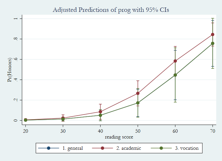
Before moving on to interactions, let’s revisit an important point, and that is that the values of the covariates really
matter when calculating predicted probabilities. In the example below, we will first get the predicted probabilities for
female for program type 1 (“general”) when the variable read is held at 30, 50 and 70. In the next example,
the values of read will be held at 31, 52 and 73. Notice the difference in the predicted probabilities in the two
output tables. While there is no “correct” values at which to hold any predictor variable, where the variables are held will
dictate what the predicted probabilities are calculated to be.
margins female, at(read=(30 50 70) prog=1) vsquish

Adjusted predictions                            Number of obs     =        200
Model VCE    : OIM

Expression   : Pr(honors), predict()
1._at        : read            =          30
               prog            =           1
2._at        : read            =          50
               prog            =           1
3._at        : read            =          70
               prog            =           1

------------------------------------------------------------------------------
             |            Delta-method
             |     Margin   Std. Err.      z    P>|z|     [95% Conf. Interval]
-------------+----------------------------------------------------------------
  _at#female |
     1#male  |   .0046867   .0038796     1.21   0.227    -.0029172    .0122906
   1#female  |   .0137226    .009905     1.39   0.166    -.0056908     .033136
     2#male  |   .0658288   .0322765     2.04   0.041      .002568    .1290896
   2#female  |   .1723344   .0683062     2.52   0.012     .0384568    .3062121
     3#male  |    .513277     .14321     3.58   0.000     .2325905    .7939635
   3#female  |   .7570458   .1152195     6.57   0.000     .5312198    .9828718
------------------------------------------------------------------------------

margins female, at(read=(31 52 73) prog=1) vsquish

Adjusted predictions                            Number of obs     =        200
Model VCE    : OIM

Expression   : Pr(honors), predict()
1._at        : read            =          31
               prog            =           1
2._at        : read            =          52
               prog            =           1
3._at        : read            =          73
               prog            =           1

------------------------------------------------------------------------------
             |            Delta-method
             |     Margin   Std. Err.      z    P>|z|     [95% Conf. Interval]
-------------+----------------------------------------------------------------
  _at#female |
     1#male  |    .005362   .0043319     1.24   0.216    -.0031284    .0138525
   1#female  |   .0156793   .0110124     1.42   0.155    -.0059045    .0372632
     2#male  |   .0845533   .0394435     2.14   0.032     .0072454    .1618611
   2#female  |   .2144007   .0798098     2.69   0.007     .0579765     .370825
     3#male  |   .6127719   .1457039     4.21   0.000     .3271974    .8983464
   3#female  |   .8238147     .09816     8.39   0.000     .6314247    1.016205
------------------------------------------------------------------------------
Models with interactions
Categorical by categorical interactions
We will start with a categorical-by-categorical interaction with the variables female and prog. First,
let’s do a three-way crosstab.
table honors female prog

--------------------------------------------------------------------------------------
                |                      type of program and female
                | ---- 1. general ----    ---- 2. academic ---    ---- 3. vocation ---
 honors english |   0. male  1. female      0. male  1. female      0. male  1. female
----------------+---------------------------------------------------------------------
0. not enrolled |        19         19           32         33           22         22
    1. enrolled |         2          5           15         25            1          5
--------------------------------------------------------------------------------------
Notice that some of the cells have very few observations.
logit honors i.female##i.prog

Iteration 0:   log likelihood = -115.64441
Iteration 1:   log likelihood = -105.80227
Iteration 2:   log likelihood = -105.03687
Iteration 3:   log likelihood = -105.01869
Iteration 4:   log likelihood = -105.01869

Logistic regression                             Number of obs     =        200
                                                LR chi2(5)        =      21.25
                                                Prob > chi2       =     0.0007
Log likelihood = -105.01869                     Pseudo R2         =     0.0919

----------------------------------------------------------------------------------
          honors |      Coef.   Std. Err.      z    P>|z|     [95% Conf. Interval]
-----------------+----------------------------------------------------------------
          female |
         female  |   .9162888   .8973641     1.02   0.307    -.8425125     2.67509
                 |
            prog |
       academic  |   1.493604   .8065652     1.85   0.064    -.0872346    3.074443
       vocation  |  -.8397523   1.264154    -0.66   0.507    -3.317448    1.637944
                 |
     female#prog |
female#academic  |  -.4362348   .9866519    -0.44   0.658    -2.370037    1.497567
female#vocation  |   .6931488   1.447816     0.48   0.632    -2.144518    3.530816
                 |
           _cons |   -2.25129   .7433913    -3.03   0.002     -3.70831   -.7942696
----------------------------------------------------------------------------------
While the overall model is statistically significant (p = 0.0007), none of the predictors are.
We will use the contrast command to get the multi-degree-of-freedom test of the interaction term, which will have 2 degrees of freedom (1*2 = 2).
contrast female#prog

Contrasts of marginal linear predictions

Margins      : asbalanced

------------------------------------------------
             |         df        chi2     P>chi2
-------------+----------------------------------
 female#prog |          2        0.97     0.6150
------------------------------------------------
The p-value for the omnibus test is 0.6150, which is well above 0.05, so the interaction term is not statistically significant. Despite these results, we
will continue to look at the interaction as if it was of interest.
We can use the margins command to give us the predicted probabilities for each combination of values of female and prog.
margins female#prog

Adjusted predictions                            Number of obs     =        200
Model VCE    : OIM

Expression   : Pr(honors), predict()

----------------------------------------------------------------------------------
                 |            Delta-method
                 |     Margin   Std. Err.      z    P>|z|     [95% Conf. Interval]
-----------------+----------------------------------------------------------------
     female#prog |
   male#general  |   .0952383   .0640565     1.49   0.137    -.0303102    .2207867
  male#academic  |   .3191489   .0679945     4.69   0.000     .1858822    .4524157
  male#vocation  |   .0434783   .0425226     1.02   0.307    -.0398645     .126821
 female#general  |   .2083333   .0828982     2.51   0.012     .0458559    .3708108
female#academic  |   .4310345   .0650257     6.63   0.000     .3035865    .5584825
female#vocation  |   .1851852   .0747568     2.48   0.013     .0386646    .3317058
----------------------------------------------------------------------------------
The predicted probabilities are rather similar for each combination of levels of the variables, which corresponds to the
fact that the interaction term is not statistically significant. We can graph the interaction with the marginsplot command.
marginsplot

  Variables that uniquely identify margins: female prog
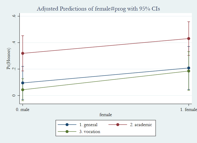
Despite the fact that the interaction is not statistically significant, we will show how some of the post-estimation commands
can be used to explore the interaction. We can get all pairwise comparisons with the pwcompare command. With no options,
we get the contrast coefficient, its standard error and its unadjusted 95% confidence interval.
pwcompare female#prog

Pairwise comparisons of marginal linear predictions

Margins      : asbalanced

-----------------------------------------------------------------------------------------------------
                                                    |                                 Unadjusted
                                                    |   Contrast   Std. Err.     [95% Conf. Interval]
----------------------------------------------------+------------------------------------------------
honors                                              |
                                        female#prog |
     (0. male#2. academic) vs (0. male#1. general)  |   .5559416   .5053125     -.4344527    1.546336
     (0. male#3. vocation) vs (0. male#1. general)  |   .0016408   .6611702     -1.294229     1.29751
    (1. female#1. general) vs (0. male#1. general)  |    1.08343   .4094357      .2809511    1.885909
   (1. female#2. academic) vs (0. male#1. general)  |   1.639372   .6280644      .4083882    2.870356
   (1. female#3. vocation) vs (0. male#1. general)  |   1.085071   .7588425     -.4022329    2.572375
    (0. male#3. vocation) vs (0. male#2. academic)  |  -.5543008    .559331     -1.650569    .5419677
   (1. female#1. general) vs (0. male#2. academic)  |   .5274886   .6719313     -.7894726     1.84445
  (1. female#2. academic) vs (0. male#2. academic)  |    1.08343   .4094357      .2809511    1.885909
  (1. female#3. vocation) vs (0. male#2. academic)  |   .5291294    .692864      -.828859    1.887118
   (1. female#1. general) vs (0. male#3. vocation)  |   1.081789   .7960686     -.4784762    2.642055
  (1. female#2. academic) vs (0. male#3. vocation)  |   1.637731   .6934817      .2785318     2.99693
  (1. female#3. vocation) vs (0. male#3. vocation)  |    1.08343   .4094357      .2809511    1.885909
 (1. female#2. academic) vs (1. female#1. general)  |   .5559416   .5053125     -.4344527    1.546336
 (1. female#3. vocation) vs (1. female#1. general)  |   .0016408   .6611702     -1.294229     1.29751
(1. female#3. vocation) vs (1. female#2. academic)  |  -.5543008    .559331     -1.650569    .5419677
-----------------------------------------------------------------------------------------------------
We can add the pveffects option to get the z test statistic and the unadjusted p-value.
pwcompare female#prog, pveffects

Pairwise comparisons of marginal linear predictions

Margins      : asbalanced

--------------------------------------------------------------------------------------------
                                                    |                            Unadjusted
                                                    |   Contrast   Std. Err.      z    P>|z|
----------------------------------------------------+---------------------------------------
honors                                              |
                                        female#prog |
     (0. male#2. academic) vs (0. male#1. general)  |   .5559416   .5053125     1.10   0.271
     (0. male#3. vocation) vs (0. male#1. general)  |   .0016408   .6611702     0.00   0.998
    (1. female#1. general) vs (0. male#1. general)  |    1.08343   .4094357     2.65   0.008
   (1. female#2. academic) vs (0. male#1. general)  |   1.639372   .6280644     2.61   0.009
   (1. female#3. vocation) vs (0. male#1. general)  |   1.085071   .7588425     1.43   0.153
    (0. male#3. vocation) vs (0. male#2. academic)  |  -.5543008    .559331    -0.99   0.322
   (1. female#1. general) vs (0. male#2. academic)  |   .5274886   .6719313     0.79   0.432
  (1. female#2. academic) vs (0. male#2. academic)  |    1.08343   .4094357     2.65   0.008
  (1. female#3. vocation) vs (0. male#2. academic)  |   .5291294    .692864     0.76   0.445
   (1. female#1. general) vs (0. male#3. vocation)  |   1.081789   .7960686     1.36   0.174
  (1. female#2. academic) vs (0. male#3. vocation)  |   1.637731   .6934817     2.36   0.018
  (1. female#3. vocation) vs (0. male#3. vocation)  |    1.08343   .4094357     2.65   0.008
 (1. female#2. academic) vs (1. female#1. general)  |   .5559416   .5053125     1.10   0.271
 (1. female#3. vocation) vs (1. female#1. general)  |   .0016408   .6611702     0.00   0.998
(1. female#3. vocation) vs (1. female#2. academic)  |  -.5543008    .559331    -0.99   0.322
--------------------------------------------------------------------------------------------
We can use the mcompare option to correct for multiple tests. In the example below, we request a Bonferroni correction.
Other possible corrections are sidak, scheffe and snk (Student-Newman-Keuls’).
pwcompare female#prog, pveffects mcompare(bon)
Pairwise comparisons of marginal linear predictions

Margins      : asbalanced

---------------------------
             |    Number of
             |  Comparisons
-------------+-------------
honors       |
 female#prog |           15
---------------------------

--------------------------------------------------------------------------------------------
                                                    |                            Bonferroni
                                                    |   Contrast   Std. Err.      z    P>|z|
----------------------------------------------------+---------------------------------------
honors                                              |
                                        female#prog |
     (0. male#2. academic) vs (0. male#1. general)  |   1.493604   .8065652     1.85   0.961
     (0. male#3. vocation) vs (0. male#1. general)  |  -.8397523   1.264154    -0.66   1.000
    (1. female#1. general) vs (0. male#1. general)  |   .9162888   .8973641     1.02   1.000
   (1. female#2. academic) vs (0. male#1. general)  |   1.973658   .7892615     2.50   0.186
   (1. female#3. vocation) vs (0. male#1. general)  |   .7696853   .8933562     0.86   1.000
    (0. male#3. vocation) vs (0. male#2. academic)  |  -2.333356   1.069285    -2.18   0.436
   (1. female#1. general) vs (0. male#2. academic)  |  -.5773154   .5920711    -0.98   1.000
  (1. female#2. academic) vs (0. male#2. academic)  |    .480054   .4101459     1.17   1.000
  (1. female#3. vocation) vs (0. male#2. academic)  |  -.7239188   .5859788    -1.24   1.000
   (1. female#1. general) vs (0. male#3. vocation)  |   1.756041   1.139336     1.54   1.000
  (1. female#2. academic) vs (0. male#3. vocation)  |    2.81341   1.056294     2.66   0.116
  (1. female#3. vocation) vs (0. male#3. vocation)  |   1.609438   1.136182     1.42   1.000
 (1. female#2. academic) vs (1. female#1. general)  |   1.057369   .5682734     1.86   0.942
 (1. female#3. vocation) vs (1. female#1. general)  |  -.1466035   .7057522    -0.21   1.000
(1. female#3. vocation) vs (1. female#2. academic)  |  -1.203973   .5619231    -2.14   0.482
--------------------------------------------------------------------------------------------
In the example below, we will use the margins command to see if female is statistically significant at each level of prog.
* contrast of adjusted predictions
margins female@prog

Contrasts of adjusted predictions
Model VCE    : OIM

Expression   : Pr(honors), predict()

------------------------------------------------
             |         df        chi2     P>chi2
-------------+----------------------------------
 female@prog |
    general  |          1        1.17     0.2804
   academic  |          1        1.41     0.2344
   vocation  |          1        2.71     0.0994
      Joint  |          3        5.29     0.1515
------------------------------------------------
If you want to make specific comparisons, you need to access the values stored either by the model or by margins.
We will start by asking if prog level 2 is different from prog level 1 for females only.
We will start by using the output from margins with the lincom command. Before we do this, let’s quietly
rerun our logistic regression model. In “Stata speak”, to run something quietly means that the model will run but no output will be shown.
This is useful when you need to be sure that the correct model is in memory, but you don’t need to see the output. Next, we will run the
margins command with the coeflegend and the post options. The coeflegend option is super useful and works with many estimation commands.
It shows you want Stata calls each of the estimates, so that you can use those estimates in post-estimation commands. The post option
posts the results to Stata’s memory so that they can be used in further calculations. You must use the post option when you use the coeflegend option with margins.
quietly logit honors i.female##i.prog
margins female#prog, coeflegend post

Adjusted predictions                            Number of obs     =        200
Model VCE    : OIM

Expression   : Pr(honors), predict()

----------------------------------------------------------------------------------
                 |     Margin  Legend
-----------------+----------------------------------------------------------------
     female#prog |
   male#general  |   .0952383  _b[0bn.female#1bn.prog]
  male#academic  |   .3191489  _b[0bn.female#2.prog]
  male#vocation  |   .0434783  _b[0bn.female#3.prog]
 female#general  |   .2083333  _b[1.female#1bn.prog]
female#academic  |   .4310345  _b[1.female#2.prog]
female#vocation  |   .1851852  _b[1.female#3.prog]
----------------------------------------------------------------------------------
lincom _b[1.female#2.prog] - _b[1.female#1bn.prog]

 ( 1)  - 1.female#1bn.prog + 1.female#2.prog = 0

------------------------------------------------------------------------------
             |      Coef.   Std. Err.      z    P>|z|     [95% Conf. Interval]
-------------+----------------------------------------------------------------
         (1) |   .2227011   .1053587     2.11   0.035      .016202    .4292003
------------------------------------------------------------------------------
Just to be sure that Stata did what we wanted, we can use the display command to calculate the value ourselves.
di .4310345  - .2083333
.2227012
The mlincom command is a convenience command that works after the margins command and is part of the spost ado package.
Instead of specifying the labels Stata assigned to each estimate, you can use the number of the estimate. First, let’s look at the matrix
of stored estimates with the matlist command.
matlist e(b)

             |  0.female#  0.female#  0.female#  1.female#  1.female#  1.female#
             |    1.prog     2.prog     3.prog     1.prog     2.prog     3.prog
-------------+------------------------------------------------------------------
          y1 |  .0952383   .3191489   .0434783   .2083333   .4310345   .1851852

mlincom 5 - 4, all

             |   lincom        se    zvalue    pvalue        ll        ul
-------------+------------------------------------------------------------
           1 |    0.223     0.105     2.114     0.035     0.016     0.429
The listcoef command can also be used. We will quietly rerun the model.
quietly logit honors i.female##i.prog

listcoef, help

logit (N=200): Factor change in odds

  Odds of: 1. enrolled vs 0. not enrolled

------------------------------------------------------------------------
             |         b        z    P>|z|       e^b   e^bStdX     SDofX
-------------+----------------------------------------------------------
      female |
  1. female  |    0.9163    1.021    0.307     2.500     1.580     0.499
             |
        prog |
2. academic  |    1.4936    1.852    0.064     4.453     2.112     0.501
3. vocation  |   -0.8398   -0.664    0.507     0.432     0.695     0.434
             |
female#c.2~g |
  1. female  |   -0.4362   -0.442    0.658     0.646     0.820     0.455
             |
female#c.3~g |
  1. female  |    0.6931    0.479    0.632     2.000     1.268     0.343
             |
    constant |   -2.2513   -3.028    0.002         .         .         .
------------------------------------------------------------------------
       b = raw coefficient
       z = z-score for test of b=0
   P>|z| = p-value for z-test
     e^b = exp(b) = factor change in odds for unit increase in X
 e^bStdX = exp(b*SD of X) = change in odds for SD increase in X
   SDofX = standard deviation of X
Categorical by continuous interactions
For this example, we will interact the binary variable female with the continuous variable socst. Let’s use the summarize
command to get some descriptive statistics on our variables.
sum i.female##c.socst

    Variable |        Obs        Mean    Std. Dev.       Min        Max
-------------+---------------------------------------------------------
      female |
  1. female  |        200        .545    .4992205          0          1
       socst |        200      52.405    10.73579         26         71
             |
      female#|
     c.socst |
  1. female  |        200       28.84    27.47231          0         71
This output is useful for many reasons. One reason is that you need to know the minimum and maximum of variables when you run the margins command.
logit honors i.female##c.socst

Iteration 0:   log likelihood = -115.64441
Iteration 1:   log likelihood = -97.381142
Iteration 2:   log likelihood = -94.500287
Iteration 3:   log likelihood = -94.374577
Iteration 4:   log likelihood = -94.374049
Iteration 5:   log likelihood = -94.374049

Logistic regression                             Number of obs     =        200
                                                LR chi2(3)        =      42.54
                                                Prob > chi2       =     0.0000
Log likelihood = -94.374049                     Pseudo R2         =     0.1839

--------------------------------------------------------------------------------
        honors |      Coef.   Std. Err.      z    P>|z|     [95% Conf. Interval]
---------------+----------------------------------------------------------------
        female |
       female  |   6.406617   3.162921     2.03   0.043     .2074054    12.60583
         socst |   .1774272   .0468628     3.79   0.000     .0855779    .2692765
               |
female#c.socst |
       female  |  -.0974514    .052999    -1.84   0.066    -.2013275    .0064248
               |
         _cons |   -11.5045   2.838154    -4.05   0.000    -17.06718   -5.941824
--------------------------------------------------------------------------------
The overall model is statistically significant (p = 0.0000), and the interaction is not significant. However, we are going to
pretend that it is and explore ways to understand the interaction. Because the interaction term has only 1 degree of freedom,
running the contrast command on the interaction is unnecessary. However, it is shown below so that you can see how to specify a
continuous variable in the command. Notice that there is only one # and the c. before the variable socst.
contrast female#c.socst

Contrasts of marginal linear predictions

Margins      : asbalanced

--------------------------------------------------
               |         df        chi2     P>chi2
---------------+----------------------------------
female#c.socst |          1        3.38     0.0660
--------------------------------------------------
The margins command can be used to get predicted probabilities for female at the desired values of socst.
margins female, at(socst=(30(20)70)) vsquish

Adjusted predictions                            Number of obs     =        200
Model VCE    : OIM

Expression   : Pr(honors), predict()

1._at        : socst           =          30
2._at        : socst           =          50
3._at        : socst           =          70

------------------------------------------------------------------------------
             |            Delta-method
             |     Margin   Std. Err.      z    P>|z|     [95% Conf. Interval]
-------------+----------------------------------------------------------------
  _at#female |
     1#male  |   .0020627   .0029825     0.69   0.489    -.0037829    .0079083
   1#female  |   .0630553    .039731     1.59   0.113     -.014816    .1409267
     2#male  |   .0670355   .0356569     1.88   0.060    -.0028507    .1369217
   2#female  |   .2499094   .0486082     5.14   0.000     .1546392    .3451797
     3#male  |   .7141036   .1132276     6.31   0.000     .4921816    .9360257
   3#female  |   .6225583   .0975773     6.38   0.000     .4313102    .8138064
------------------------------------------------------------------------------
The values in this table can be graphed with the marginsplot command.
marginsplot

  Variables that uniquely identify margins: socst female
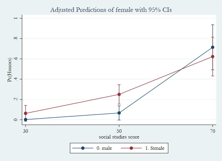
As before, we can make comparisons between the values calculated by margins. Notice, however, that the variable read is
still a continuous variable in the model, even though we can test difference at different values.
margins female, at(socst=(30(20)70)) coeflegend post vsquish

Adjusted predictions                            Number of obs     =        200
Model VCE    : OIM

Expression   : Pr(honors), predict()

1._at        : socst           =          30
2._at        : socst           =          50
3._at        : socst           =          70

------------------------------------------------------------------------------
             |     Margin  Legend
-------------+----------------------------------------------------------------
  _at#female |
     1#male  |   .0020627  _b[1bn._at#0bn.female]
   1#female  |   .0630553  _b[1bn._at#1.female]
     2#male  |   .0670355  _b[2._at#0bn.female]
   2#female  |   .2499094  _b[2._at#1.female]
     3#male  |   .7141036  _b[3._at#0bn.female]
   3#female  |   .6225583  _b[3._at#1.female]
------------------------------------------------------------------------------
Let’s test the difference between females and males when the social study score is 50.
lincom _b[2._at#1.female] - _b[2._at#0bn.female]

 ( 1)  - 2._at#0bn.female + 2._at#1.female = 0

------------------------------------------------------------------------------
             |      Coef.   Std. Err.      z    P>|z|     [95% Conf. Interval]
-------------+----------------------------------------------------------------
         (1) |    .182874   .0602841     3.03   0.002     .0647194    .3010285
------------------------------------------------------------------------------
This difference is statistically significant. Now let’s do the same test when the social studies score is 30.
lincom _b[1._at#1.female] - _b[1._at#0bn.female]

 ( 1)  - 1bn._at#0bn.female + 1bn._at#1.female = 0

------------------------------------------------------------------------------
             |      Coef.   Std. Err.      z    P>|z|     [95% Conf. Interval]
-------------+----------------------------------------------------------------
         (1) |   .0609926   .0398428     1.53   0.126    -.0170978    .1390831
------------------------------------------------------------------------------
At this value of socst, the difference between females and males is not statistically significantly different.
Before moving on to continuous by continuous interactions, let’s stop and add one more continuous predictor to our model.
We will add the variable read and show how the predicted probabilities change when read is held at different values.
logit honors i.female##c.socst read

Iteration 0:   log likelihood = -115.64441
Iteration 1:   log likelihood = -86.134978
Iteration 2:   log likelihood = -82.031517
Iteration 3:   log likelihood = -81.860765
Iteration 4:   log likelihood = -81.859756
Iteration 5:   log likelihood = -81.859756

Logistic regression                             Number of obs     =        200
                                                LR chi2(4)        =      67.57
                                                Prob > chi2       =     0.0000
Log likelihood = -81.859756                     Pseudo R2         =     0.2921

--------------------------------------------------------------------------------
        honors |      Coef.   Std. Err.      z    P>|z|     [95% Conf. Interval]
---------------+----------------------------------------------------------------
        female |
    1. female  |    7.12505   3.113835     2.29   0.022     1.022045    13.22805
         socst |   .1084125   .0469643     2.31   0.021     .0163642    .2004608
               |
female#c.socst |
    1. female  |  -.1049667   .0525745    -2.00   0.046    -.2080107   -.0019226
               |
          read |     .12548   .0277186     4.53   0.000     .0711525    .1798076
         _cons |  -14.76649   2.955381    -5.00   0.000    -20.55893   -8.974047
--------------------------------------------------------------------------------
This output looks good. Now let’s use the margins command and include only the at option to specify levels of socst.
The default is for Stata to treat other variables in the model as their values are observed. The asobserved option can be added to produce the
same results.
margins female, at(socst=(30(20)70))

Predictive margins                              Number of obs     =        200
Model VCE    : OIM

Expression   : Pr(honors), predict()

1._at        : socst           =          30

2._at        : socst           =          50

3._at        : socst           =          70

------------------------------------------------------------------------------
             |            Delta-method
             |     Margin   Std. Err.      z    P>|z|     [95% Conf. Interval]
-------------+----------------------------------------------------------------
  _at#female |
  1#0. male  |   .0150025   .0208116     0.72   0.471    -.0257876    .0557925
1#1. female  |     .32096   .1268867     2.53   0.011     .0722666    .5696534
  2#0. male  |   .1010581   .0439717     2.30   0.022     .0148752     .187241
2#1. female  |   .3322728   .0470899     7.06   0.000     .2399783    .4245674
  3#0. male  |   .3819052   .1132221     3.37   0.001     .1599939    .6038165
3#1. female  |   .3437552   .0826705     4.16   0.000      .181724    .5057863
------------------------------------------------------------------------------

margins female, at(socst=(30(20)70)) asobserved

Predictive margins                              Number of obs     =        200
Model VCE    : OIM

Expression   : Pr(honors), predict()

1._at        : socst           =          30

2._at        : socst           =          50

3._at        : socst           =          70

------------------------------------------------------------------------------
             |            Delta-method
             |     Margin   Std. Err.      z    P>|z|     [95% Conf. Interval]
-------------+----------------------------------------------------------------
  _at#female |
  1#0. male  |   .0150025   .0208116     0.72   0.471    -.0257876    .0557925
1#1. female  |     .32096   .1268867     2.53   0.011     .0722666    .5696534
  2#0. male  |   .1010581   .0439717     2.30   0.022     .0148752     .187241
2#1. female  |   .3322728   .0470899     7.06   0.000     .2399783    .4245674
  3#0. male  |   .3819052   .1132221     3.37   0.001     .1599939    .6038165
3#1. female  |   .3437552   .0826705     4.16   0.000      .181724    .5057863
------------------------------------------------------------------------------
Now let’s set the value of read to its mean.
margins female, at(socst=(30(20)70) read = (52.23))

Adjusted predictions                            Number of obs     =        200
Model VCE    : OIM

Expression   : Pr(honors), predict()

1._at        : socst           =          30
               read            =       52.23

2._at        : socst           =          50
               read            =       52.23

3._at        : socst           =          70
               read            =       52.23

------------------------------------------------------------------------------
             |            Delta-method
             |     Margin   Std. Err.      z    P>|z|     [95% Conf. Interval]
-------------+----------------------------------------------------------------
  _at#female |
  1#0. male  |   .0069621   .0096717     0.72   0.472    -.0119941    .0259182
1#1. female  |   .2720513   .1463304     1.86   0.063     -.014751    .5588535
  2#0. male  |   .0577558   .0308495     1.87   0.061     -.002708    .1182197
2#1. female  |   .2859118   .0551228     5.19   0.000     .1778731    .3939505
  3#0. male  |   .3489201    .152427     2.29   0.022     .0501687    .6476715
3#1. female  |   .3001873   .1109357     2.71   0.007     .0827573    .5176174
------------------------------------------------------------------------------
Now let’s set the value of read to 60.
margins female, at(socst=(30(20)70) read = (60))

Adjusted predictions                            Number of obs     =        200
Model VCE    : OIM

Expression   : Pr(honors), predict()

1._at        : socst           =          30
               read            =          60

2._at        : socst           =          50
               read            =          60

3._at        : socst           =          70
               read            =          60

------------------------------------------------------------------------------
             |            Delta-method
             |     Margin   Std. Err.      z    P>|z|     [95% Conf. Interval]
-------------+----------------------------------------------------------------
  _at#female |
  1#0. male  |   .0182475   .0255591     0.71   0.475    -.0318473    .0683423
1#1. female  |    .497685   .2124644     2.34   0.019     .0812624    .9141075
  2#0. male  |    .139787   .0673932     2.07   0.038     .0076987    .2718754
2#1. female  |   .5149098   .0878009     5.86   0.000     .3428232    .6869964
  3#0. male  |   .5869062   .1449033     4.05   0.000      .302901    .8709114
3#1. female  |   .5320993   .1124178     4.73   0.000     .3117644    .7524342
------------------------------------------------------------------------------
The output in the last two tables is different, even though the variable read was not included in the interaction. This
is why we say that the value of the covariates matter when calculating the predicted probabilities. Of course, in the metric of log odds,
the value at which read is held does not matter when calculating the coefficients of the other variables.
Continuous by continuous interactions
For this example, we will interact the variables read and science. First, let’s look at some descriptive statistics.
sum c.read##c.science

    Variable |        Obs        Mean    Std. Dev.       Min        Max
-------------+---------------------------------------------------------
        read |        200       52.23    10.25294         28         76
     science |        200       51.85    9.900891         26         74
             |
      c.read#|
   c.science |        200    2771.775    952.0686        986       5092
Now we will run our model.
logit honors c.read##c.science

Iteration 0:   log likelihood = -115.64441
Iteration 1:   log likelihood =   -89.3918
Iteration 2:   log likelihood = -85.086047
Iteration 3:   log likelihood = -84.668677
Iteration 4:   log likelihood = -84.666101
Iteration 5:   log likelihood = -84.666101

Logistic regression                             Number of obs     =        200
                                                LR chi2(3)        =      61.96
                                                Prob > chi2       =     0.0000
Log likelihood = -84.666101                     Pseudo R2         =     0.2679

----------------------------------------------------------------------------------
          honors |      Coef.   Std. Err.      z    P>|z|     [95% Conf. Interval]
-----------------+----------------------------------------------------------------
            read |   .3965415   .1728687     2.29   0.022     .0577252    .7353579
         science |   .3480727   .1646122     2.11   0.034     .0254387    .6707068
                 |
c.read#c.science |  -.0051357   .0029119    -1.76   0.078    -.0108429    .0005715
                 |
           _cons |  -26.28497   9.642589    -2.73   0.006     -45.1841   -7.385845
----------------------------------------------------------------------------------
By now you should be feeling pretty comfortable with the basics of the output above. So let’s start with a seemingly easy question:
Is the interaction term statistically significant? Many people would say no because the observed p-value of 0.078 is greater than our alpha level
of 0.05. However, this is one of the places where logistic regression and OLS regression are not similar at all.
Here is a quote from Norton, Wang and Ai (2004):
“Unfortunately, the intuition from linear regression models does not ex-tend to nonlinear models. The marginal effect of a change in both interacted
variables is not equal to the marginal effect of changing just the interaction term. More surprisingly, the sign may be different for different observations.
The statistical significance cannot be determined from the z-statistic reported in the regression output. The odds-ratio interpretation of logit coefficients
cannot be used for interaction terms.” (page 154)
“There are four important implications of this equation for nonlinear models. First,the interaction effect could be nonzero, even if ß12 = 0. Second,
the statistical significance of the interaction effect cannot be tested with a simple t test on the coefficient of the interaction term ß12. Instead,
the statistical significance of the entire cross derivative must be calculated. Third, the interaction effect is conditional on the independent
variables, unlike the interaction effect in linear models. (It is well known that the marginal effect of a single, uninteracted variable in a
nonlinear model is conditional on the independent variables.) Fourth, because there are two additive terms, each of which can be positive or negative,
the interaction effect may have different signs for different values of covariates. Therefore, the sign of ß12 does not necessarily indicate
the sign of the interaction effect.” (page 156)
What this means for reporting your results is that you should not state whether your interaction is statistically significant. Rather, you will need to discuss one
or more ranges in which the interaction is statistically significant, regardless of the p-value given in the output table.
We will use Norton, et. al.’s inteff command to examine the interaction. The inteff command requires that you create the interaction term manually and run the logit command
with that interaction term before inteff.
gen readsci = read*science

quietly logit honors read science readsci

inteff honors read science readsci

Logit with two continuous variables interacted

    Variable |        Obs        Mean    Std. Dev.       Min        Max
-------------+---------------------------------------------------------
   _logit_ie |        200   -.0002656    .0007018  -.0013207   .0005851
   _logit_se |        200    .0004389    .0002959   .0000202   .0011699
    _logit_z |        200    .6022096    2.153007  -2.710142   4.456493
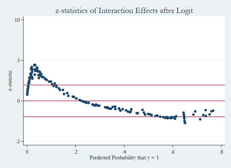
The graph shows two regions where the interaction is statistically significant. Another community-contributed command called inteff3 can be used when a
binary by binary by binary interaction is used (difference-in-difference-in-difference).
There are a couple of articles that provide helpful examples of correctly interpreting interactions in non-linear models. One is by Maarten Buis (referenced below), and another is a post by Vince Wiggins of Stata Corp.
Despite the difficulties of knowing if or where the interaction term is statistically significant, and not being able to interpret the odds ratio of the interaction term, we can still use the margins command to get some descriptive information about the interaction. This can be done because we are not talking about statistical significance; rather, we are only looking at descriptive values based on the current model. We will quietly rerun the model in a way that margins will understand.
quietly logit honors c.read##c.science
margins, at(read=(30(20)70) science=(30 50 70)) vsquish

Adjusted predictions                            Number of obs     =        200
Model VCE    : OIM

Expression   : Pr(honors), predict()
1._at        : read            =          30
               science         =          30
2._at        : read            =          30
               science         =          50
3._at        : read            =          30
               science         =          70
4._at        : read            =          50
               science         =          30
5._at        : read            =          50
               science         =          50
6._at        : read            =          50
               science         =          70
7._at        : read            =          70
               science         =          30
8._at        : read            =          70
               science         =          50
9._at        : read            =          70
               science         =          70

------------------------------------------------------------------------------
             |            Delta-method
             |     Margin   Std. Err.      z    P>|z|     [95% Conf. Interval]
-------------+----------------------------------------------------------------
         _at |
          1  |   .0001899   .0004304     0.44   0.659    -.0006536    .0010334
          2  |   .0091155   .0081189     1.12   0.262    -.0067972    .0250283
          3  |   .3081947    .267849     1.15   0.250    -.2167798    .8331691
          4  |   .0236781   .0196095     1.21   0.227    -.0147557     .062112
          5  |   .1308492   .0349136     3.75   0.000     .0624198    .1992785
          6  |    .483081   .1363859     3.54   0.000     .2157696    .7503924
          7  |   .7558718   .2854873     2.65   0.008      .196327    1.315417
          8  |   .7112934   .1261598     5.64   0.000     .4640247    .9585621
          9  |   .6622125   .1319474     5.02   0.000     .4036003    .9208247
------------------------------------------------------------------------------
marginsplot, legend(rows(1))

  Variables that uniquely identify margins: read science
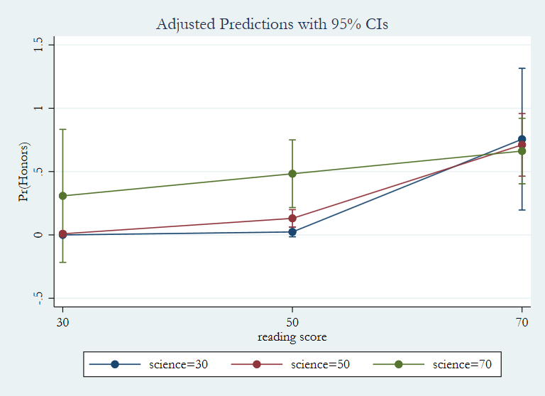
Let’s look at one last example. This time we will use the square of reading score as the interaction term.
*logit honors c.read##c.read
gen read2 = read*read
logit honors read read read2

note: read omitted because of collinearity
Iteration 0:   log likelihood = -115.64441
Iteration 1:   log likelihood = -91.768787
Iteration 2:   log likelihood =  -88.71512
Iteration 3:   log likelihood = -88.475651
Iteration 4:   log likelihood = -88.474528
Iteration 5:   log likelihood = -88.474527

Logistic regression                             Number of obs     =        200
                                                LR chi2(2)        =      54.34
                                                Prob > chi2       =     0.0000
Log likelihood = -88.474527                     Pseudo R2         =     0.2349

------------------------------------------------------------------------------
      honors |      Coef.   Std. Err.      z    P>|z|     [95% Conf. Interval]
-------------+----------------------------------------------------------------
        read |   .5116124   .2741212     1.87   0.062    -.0256554     1.04888
        read |          0  (omitted)
       read2 |   -.003321   .0023626    -1.41   0.160    -.0079516    .0013096
       _cons |  -18.88234   7.849826    -2.41   0.016    -34.26771   -3.496961
------------------------------------------------------------------------------

inteff honors read read read2
Logit with two continuous variables interacted

    Variable |        Obs        Mean    Std. Dev.       Min        Max
-------------+---------------------------------------------------------
   _logit_ie |        200    .0039721    .0055833  -.0064616   .0106083
   _logit_se |        200    .0018632    .0008679   .0002302   .0041644
    _logit_z |        200    3.559618    4.169944  -2.229903   10.73907
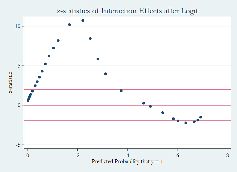
As before, we see that the p-value in the logistic regression output indicates that the interaction term is not statistically significant, yet it seems that for some regions, the interaction is statistically significant. This is why such interaction terms are so difficult in logistic regression.
References
Buis, M. L. (2010). Stata Tip 87: Interpretation of interactions in nonlinear models. The Stata Journal, 10(2), pages 305-308.
Hosmer, D. W., Lemeshow, S. and Sturdivant, R. X. (2013). Applied Logistic Regression, Third Edition. Hoboken, New Jersey: Wiley.
Long, J. S. and Freese, J. (2014). Regression Models for Categorical Dependent Variables Using Stata, Third Edition. College Station, TX: Stata Press.
Norton, E. C., Wang, H., and Ai, C. (2004). Computing interaction effects and standard errors in logit and probit models. The Stata Journal, 4(2), pages 154-167.
Williams, R. (2012). Using the margins command to estimate and interpret adjusted predictions and marginal effects. The Stata Journal, 12(2), pages 308-331.