
1.
Use the crime data file that was used in chapter 2 (use https://stats.idre.ucla.edu/stat/stata/webbooks/reg/crime ) and look at a regression model
predicting murder from pctmetro, poverty, pcths and single
using OLS and make a avplots and a lvr2plot following
the regression. Are there any states that look worrisome? Repeat this analysis using
regression with robust standard errors and show avplots for the analysis.
Repeat the analysis using robust regression and make a manually created lvr2plot.
Also run the results using qreg. Compare the results of the different
analyses. Look at the weights from the robust regression and comment on the weights.
Answer 1.
First, consider the OLS regression predicting murder from pctmetro,
poverty, pcths and single.
use https://stats.idre.ucla.edu/stat/stata/webbooks/reg/crime , clear
(crime data from agresti & finlay - 1997)
regress murder pctmetro poverty pcths single
      Source |       SS       df       MS              Number of obs =      51
-------------+------------------------------           F(  4,    46) =   37.90
       Model |  4406.42207     4  1101.60552           Prob > F      =  0.0000
    Residual |  1336.89947    46  29.0630319           R-squared     =  0.7672
-------------+------------------------------           Adj R-squared =  0.7470
       Total |  5743.32154    50  114.866431           Root MSE      =   5.391

------------------------------------------------------------------------------
      murder |      Coef.   Std. Err.      t    P>|t|     [95% Conf. Interval]
-------------+----------------------------------------------------------------
    pctmetro |   .0682218   .0380637     1.79   0.080    -.0083964      .14484
     poverty |   .4380115   .3259862     1.34   0.186    -.2181648    1.094188
       pcths |   .0243003   .2220237     0.11   0.913    -.4226102    .4712109
      single |   3.650532   .4982054     7.33   0.000     2.647697    4.653367
       _cons |  -45.31188   19.39747    -2.34   0.024    -84.35697   -6.266792
------------------------------------------------------------------------------
These results suggest that single is the only predictor significantly
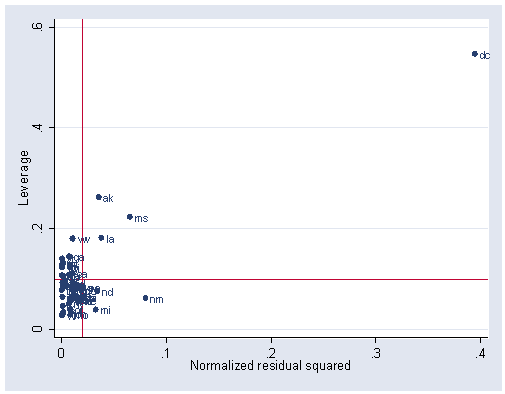
related to number of murders in a state. Let’s look at the lvr2plot for
this analysis. Washington DC looks like it has both a very high leverage and a very high
residual.
. lvr2plot, mlabel(state)
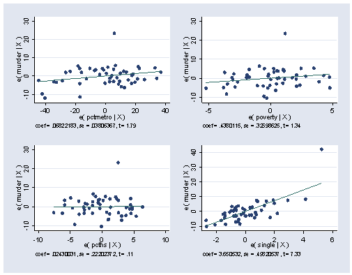
. avplots
Let’s consider the same analysis using robust standard errors. The results are largely
the same, except that the p value for pctmetro fell from 0.08 to 0.049,
which would then make it a significant predictor, however we would be somewhat skeptical
of this particular result without further investigation.
regress murder pctmetro poverty pcths single, robust
Regression with robust standard errors                 Number of obs =      51
                                                       F(  4,    46) =    7.20
                                                       Prob > F      =  0.0001
                                                       R-squared     =  0.7672
                                                       Root MSE      =   5.391

------------------------------------------------------------------------------
             |               Robust
      murder |      Coef.   Std. Err.      t    P>|t|     [95% Conf. Interval]
-------------+----------------------------------------------------------------
    pctmetro |   .0682218   .0337517     2.02   0.049     .0002832    .1361604
     poverty |   .4380115   .2568971     1.71   0.095    -.0790955    .9551185
       pcths |   .0243003   .1841403     0.13   0.896    -.3463549    .3949556
      single |   3.650532   1.152474     3.17   0.003     1.330723    5.970341
       _cons |  -45.31188   25.39531    -1.78   0.081    -96.42999    5.806231
------------------------------------------------------------------------------
Stata allows us to compute the residual for this analysis but will not allow us to
compute the leverage (hat) value. So instead of showing a lvr2plot let’s
look at the avplots for this analysis.
. avplots , mlabel(state)
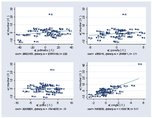
As you can see, we still have an observation that sticks out from the rest, and this is
Washington DC. This is especially pronounced for the lower right graph for single
where DC would seem to have very strong leverage to influence the coefficient for single.
Now, let’s look at the analysis using robust regression and save the weights, calling
them rrwt.
rreg murder pctmetro poverty pcths single, genwt(rrwt)
   Huber iteration 1:  maximum difference in weights = .44857261
   Huber iteration 2:  maximum difference in weights = .0399983
Biweight iteration 3:  maximum difference in weights = .15321379
Biweight iteration 4:  maximum difference in weights = .00973214

Robust regression estimates                            Number of obs =      50
                                                       F(  4,    45) =   35.25
                                                       Prob > F      =  0.0000

------------------------------------------------------------------------------
      murder |      Coef.   Std. Err.      t    P>|t|     [95% Conf. Interval]
-------------+----------------------------------------------------------------
    pctmetro |   .0535439   .0146555     3.65   0.001     .0240262    .0830615
     poverty |    .182561   .1259505     1.45   0.154    -.0711163    .4362383
       pcths |  -.2245853   .0863452    -2.60   0.013    -.3984936   -.0506771
      single |   1.392942   .2355845     5.91   0.000     .9184503    1.867434
       _cons |   2.888033   7.945302     0.36   0.718    -13.11463    18.89069
------------------------------------------------------------------------------
If you try the avplots command, this command is not available after rreg
and the lvr2plot is not available either. But we can manually create the
residual and hat values and create an lvr2plot of our own, see below.
predict r, r
predict h, hat
generate r2=r^2
sum r2
<output omitted>
replace r2 = r2/r(sum)
summarize r2
<output omitted>
local rm = r(mean)
summarize h
<output omitted>
local hm = r(mean)
graph twoway scatter h r2 if state ~= "dc", yline(`hm') xline(`rm') mlabel(state) xlabel(0(.005).025)
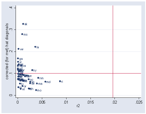
As you see above, using the robust regression, none of the observations are jointly
high in leverage and their residual values. Let’s recap the regress
results and the rreg results below and compare them.
regress murder pctmetro poverty pcths single
      Source |       SS       df       MS              Number of obs =      51
-------------+------------------------------           F(  4,    46) =   37.90
       Model |  4406.42207     4  1101.60552           Prob > F      =  0.0000
    Residual |  1336.89947    46  29.0630319           R-squared     =  0.7672
-------------+------------------------------           Adj R-squared =  0.7470
       Total |  5743.32154    50  114.866431           Root MSE      =   5.391

------------------------------------------------------------------------------
      murder |      Coef.   Std. Err.      t    P>|t|     [95% Conf. Interval]
-------------+----------------------------------------------------------------
    pctmetro |   .0682218   .0380637     1.79   0.080    -.0083964      .14484
     poverty |   .4380115   .3259862     1.34   0.186    -.2181648    1.094188
       pcths |   .0243003   .2220237     0.11   0.913    -.4226102    .4712109
      single |   3.650532   .4982054     7.33   0.000     2.647697    4.653367
       _cons |  -45.31188   19.39747    -2.34   0.024    -84.35697   -6.266792
------------------------------------------------------------------------------
rreg murder pctmetro poverty pcths single
   Huber iteration 1:  maximum difference in weights = .44857261
   Huber iteration 2:  maximum difference in weights = .0399983
Biweight iteration 3:  maximum difference in weights = .15321379
Biweight iteration 4:  maximum difference in weights = .00973214

Robust regression estimates                            Number of obs =      50
                                                       F(  4,    45) =   35.25
                                                       Prob > F      =  0.0000

------------------------------------------------------------------------------
      murder |      Coef.   Std. Err.      t    P>|t|     [95% Conf. Interval]
-------------+----------------------------------------------------------------
    pctmetro |   .0535439   .0146555     3.65   0.001     .0240262    .0830615
     poverty |    .182561   .1259505     1.45   0.154    -.0711163    .4362383
       pcths |  -.2245853   .0863452    -2.60   0.013    -.3984936   -.0506771
      single |   1.392942   .2355845     5.91   0.000     .9184503    1.867434
       _cons |   2.888033   7.945302     0.36   0.718    -13.11463    18.89069
------------------------------------------------------------------------------
The results are consistent for poverty and for single,
where poverty was not significant in both analyses and single
was significant in both analyses. However, the results for pctmetro and pcths
were both not significant in the OLS analysis and were significant in the robust
regression anlaysis.
Let’s look at the weights used in the robust regression to further understand why the
results were so different. Note that the weight for dc is .
meaning that it was eliminated from the analysis entirely (because it had such a high
residual). Also, ri was weighted by less than half.
hilo rrwt state
10 lowest and highest observations on rrwt

      rrwt      state
46982663         ri
62949383         md
716977         nm
73472243         ma
74565543         mo
75750112         la
79708217         ky
82324958         ks
82552144         de
82728266         il

      rrwt      state
99592844         sd
99639177         pa
99799356         fl
99811845         vt
99838103         ga
99863411         nh
99981867         wy
99986937         nd
99991851         ok
dc
In our analyses in chapter 2 (involving different variables) we found dc
to be a very serious outlier and decided that it should be excluded because it is not a
state. If we investigated further into these variables we may reach the same conclusion
and decide that dc should be excluded. If we did, we could try using OLS
regression like this. These results are quite similar to the rreg
results. The benefits of rreg is that it deals not only with the serious
problems (like dc being a very bad outlier) but also minor problems as
well.
regress murder pctmetro poverty pcths single if state != "dc"
      Source |       SS       df       MS              Number of obs =      50
-------------+------------------------------           F(  4,    45) =   39.88
       Model |  606.611746     4  151.652936           Prob > F      =  0.0000
    Residual |  171.137027    45  3.80304505           R-squared     =  0.7800
-------------+------------------------------           Adj R-squared =  0.7604
       Total |  777.748773    49  15.8724239           Root MSE      =  1.9501

------------------------------------------------------------------------------
      murder |      Coef.   Std. Err.      t    P>|t|     [95% Conf. Interval]
-------------+----------------------------------------------------------------
    pctmetro |   .0534333    .013795     3.87   0.000     .0256488    .0812178
     poverty |   .2237151   .1185554     1.89   0.066    -.0150679     .462498
       pcths |  -.1938711   .0812756    -2.39   0.021    -.3575685   -.0301737
      single |   1.388337   .2217525     6.26   0.000     .9417051     1.83497
       _cons |  -.0044014   7.478803    -0.00   1.000    -15.06748    15.05868
------------------------------------------------------------------------------
Let’s try running the results using qreg and compare them with rreg.
qreg murder pctmetro poverty pcths single
Iteration  1:  WLS sum of weighted deviations =  187.90652

Iteration  1: sum of abs. weighted deviations =  177.16784
Iteration  2: sum of abs. weighted deviations =  167.01302
Iteration  3: sum of abs. weighted deviations =  128.40282
Iteration  4: sum of abs. weighted deviations =  125.28249
Iteration  5: sum of abs. weighted deviations =    124.226
Iteration  6: sum of abs. weighted deviations =  122.93248
Iteration  7: sum of abs. weighted deviations =   122.6427
Iteration  8: sum of abs. weighted deviations =  122.40488
Iteration  9: sum of abs. weighted deviations =  122.03476
Iteration 10: sum of abs. weighted deviations =  122.03096

Median regression                                    Number of obs =        51
  Raw sum of deviations    235.3 (about 6.8000002)
  Min sum of deviations  122.031                     Pseudo R2     =    0.4814

------------------------------------------------------------------------------
      murder |      Coef.   Std. Err.      t    P>|t|     [95% Conf. Interval]
-------------+----------------------------------------------------------------
    pctmetro |   .0527879   .0226177     2.33   0.024     .0072608     .098315
     poverty |   .0908506   .1831176     0.50   0.622    -.2777461    .4594473
       pcths |  -.2686652   .1284197    -2.09   0.042    -.5271606   -.0101697
      single |   1.796151   .2859057     6.28   0.000     1.220652    2.371649
       _cons |   3.524669   11.34322     0.31   0.757    -19.30806    26.35739
------------------------------------------------------------------------------
rreg murder pctmetro poverty pcths single
   Huber iteration 1:  maximum difference in weights = .44857261
   Huber iteration 2:  maximum difference in weights = .0399983
Biweight iteration 3:  maximum difference in weights = .15321379
Biweight iteration 4:  maximum difference in weights = .00973214

Robust regression estimates                            Number of obs =      50
                                                       F(  4,    45) =   35.25
                                                       Prob > F      =  0.0000

------------------------------------------------------------------------------
      murder |      Coef.   Std. Err.      t    P>|t|     [95% Conf. Interval]
-------------+----------------------------------------------------------------
    pctmetro |   .0535439   .0146555     3.65   0.001     .0240262    .0830615
     poverty |    .182561   .1259505     1.45   0.154    -.0711163    .4362383
       pcths |  -.2245853   .0863452    -2.60   0.013    -.3984936   -.0506771
      single |   1.392942   .2355845     5.91   0.000     .9184503    1.867434
       _cons |   2.888033   7.945302     0.36   0.718    -13.11463    18.89069
------------------------------------------------------------------------------
While the coefficients do not always match up, the variables that were significant
in
the qreg are also significant in the rreg and likewise
for the non-significant variables. Even though these techniques use different strategies
for resisting the influence of very deviant observations, they both arrive at the same
conclusions regarding which variables are significantly related to murder,
although they do not always agree in the strength of the relationship, i.e. the size of
the coefficients.
2.
Using the elemapi2 data file (use https://stats.idre.ucla.edu/stat/stata/webbooks/reg/elemapi2 )
pretend that 550 is the lowest score that a school could achieve on api00,
i.e., create a new variable with the api00 score and recode it such that
any score of 550 or below becomes 550. Use meals, ell and
emer to predict api scores using 1) OLS to predict the original api score
(before recoding) 2) OLS to predict the recoded score where 550 was the lowest value, and
3) using tobit to predict the recoded api score indicating the lowest
value is 550. Compare the results of these analyses.
Answer 2.
First, we will use the elemapi2 data file and create the recoded version
of the api score where the lowest value is 550. We will call this value api00x.
use https://stats.idre.ucla.edu/stat/stata/webbooks/reg/elemapi2 , clear
gen api00x = api00
replace api00x = 550 if api00 <= 550
(122 real changes made)
Analysis 1. Now, we will run an OLS regression on the un-recoded version of api.
regress api00 meals ell emer
      Source |       SS       df       MS              Number of obs =     400
-------------+------------------------------           F(  3,   396) =  673.00
       Model |  6749782.75     3  2249927.58           Prob > F      =  0.0000
    Residual |  1323889.25   396  3343.15467           R-squared     =  0.8360
-------------+------------------------------           Adj R-squared =  0.8348
       Total |  8073672.00   399  20234.7669           Root MSE      =   57.82

------------------------------------------------------------------------------
       api00 |      Coef.   Std. Err.      t    P>|t|     [95% Conf. Interval]
-------------+----------------------------------------------------------------
       meals |  -3.159189   .1497371   -21.10   0.000    -3.453568   -2.864809
         ell |  -.9098732   .1846442    -4.93   0.000    -1.272878   -.5468678
        emer |  -1.573496    .293112    -5.37   0.000    -2.149746   -.9972456
       _cons |   886.7033    6.25976   141.65   0.000     874.3967    899.0098
------------------------------------------------------------------------------
Analysis 2. Now, we run an OLS regression on the recoded version of api.
regress api00x meals ell emerSource | SS df MS Number of obs = 400 -------------+------------------------------ F( 3, 396) = 682.88 Model | 4567355.46 3 1522451.82 Prob > F = 0.0000 Residual | 882862.941 396 2229.45187 R-squared = 0.8380 -------------+------------------------------ Adj R-squared = 0.8368 Total | 5450218.40 399 13659.6952 Root MSE = 47.217 ------------------------------------------------------------------------------ api00x | Coef. Std. Err. t P>|t| [95% Conf. Interval] -------------+---------------------------------------------------------------- meals | -3.010788 .1222786 -24.62 0.000 -3.251184 -2.770392 ell | -.3034092 .1507844 -2.01 0.045 -.5998472 -.0069713 emer | -.7484733 .2393616 -3.13 0.002 -1.219052 -.277895 _cons | 869.31 5.111854 170.06 0.000 859.2602 879.3597 ------------------------------------------------------------------------------
Analysis 3. And we use tobit to perform the analysis indicating that
the lowest value possible was 550.
tobit api00x meals ell emer , ll(550)
Tobit estimates                                   Number of obs   =        400
                                                  LR chi2(3)      =     660.74
                                                  Prob > chi2     =     0.0000
Log likelihood = -1581.8117                       Pseudo R2       =     0.1728

------------------------------------------------------------------------------
      api00x |      Coef.   Std. Err.      t    P>|t|     [95% Conf. Interval]
-------------+----------------------------------------------------------------
       meals |  -3.145065   .1595799   -19.71   0.000    -3.458792   -2.831337
         ell |  -.8633529    .212474    -4.06   0.000    -1.281068   -.4456381
        emer |  -1.470878   .3361215    -4.38   0.000    -2.131678   -.8100772
       _cons |   885.2395   6.372871   138.91   0.000     872.7107    897.7683
-------------+----------------------------------------------------------------
         _se |   57.12718   2.473494           (Ancillary parameter)
------------------------------------------------------------------------------

  Obs. summary:        122  left-censored observations at api00x <=550 278 uncensored observations
First, let’s compare analysis 1 and 2. When the range in api was restricted in
analysis 2, the size of the coefficients dropped due to the restriction in range of the api scores.
For example, the coefficient for ell dropped from -.9 to -.3 and its
significance level changed to 0.045 (nearly not significant from being quite significant).
Let’s see how well the tobit analysis compensated for the restriction in
range by comparing analysis #1 and #3. The coefficients are quite similar in these two
analyses. The standard errors are slightly larger in the tobit analysis
leading the t values to be somewhat smaller. Nevertheless, the tobit
estimates are much more on target than the second OLS analysis on the recoded data.
3.
Using the elemapi2 data file (use https://stats.idre.ucla.edu/stat/stata/webbooks/reg/elemapi2 )
pretend that only schools with api scores of 550 or higher were included in the sample.
Use meals ell and emer to predict api
scores using 1) OLS to predict api from the full set of observations, 2) OLS to predict
api using just the observations with api scores of 550 or higher, and 3) using truncreg
to predict api using just the observations where api is 550 or higher. Compare the results
of these analyses.
Answer 3.
First, we use the elemapi2 data file and run the analysis on the complete
data.
use https://stats.idre.ucla.edu/stat/stata/webbooks/reg/elemapi2, clear
Analysis 1 using all of the data.
regress api00 meals ell emer
      Source |       SS       df       MS              Number of obs =     400
-------------+------------------------------           F(  3,   396) =  673.00
       Model |  6749782.75     3  2249927.58           Prob > F      =  0.0000
    Residual |  1323889.25   396  3343.15467           R-squared     =  0.8360
-------------+------------------------------           Adj R-squared =  0.8348
       Total |  8073672.00   399  20234.7669           Root MSE      =   57.82

------------------------------------------------------------------------------
       api00 |      Coef.   Std. Err.      t    P>|t|     [95% Conf. Interval]
-------------+----------------------------------------------------------------
       meals |  -3.159189   .1497371   -21.10   0.000    -3.453568   -2.864809
         ell |  -.9098732   .1846442    -4.93   0.000    -1.272878   -.5468678
        emer |  -1.573496    .293112    -5.37   0.000    -2.149746   -.9972456
       _cons |   886.7033    6.25976   141.65   0.000     874.3967    899.0098
------------------------------------------------------------------------------
Now let’s keep just the schools with api scores of 550 or higher for the next 2
analyses.
keep if api00 >= 550
(122 observations deleted)
Analysis 2 using OLS on just the schools with api scores of 550 or higher.
regress api00 meals ell emer
      Source |       SS       df       MS              Number of obs =     278
-------------+------------------------------           F(  3,   274) =  292.55
       Model |  2268727.43     3  756242.478           Prob > F      =  0.0000
    Residual |  708297.044   274  2585.02571           R-squared     =  0.7621
-------------+------------------------------           Adj R-squared =  0.7595
       Total |  2977024.48   277  10747.3808           Root MSE      =  50.843

------------------------------------------------------------------------------
       api00 |      Coef.   Std. Err.      t    P>|t|     [95% Conf. Interval]
-------------+----------------------------------------------------------------
       meals |  -2.798288   .1600331   -17.49   0.000    -3.113339   -2.483238
         ell |  -.3584496   .2315111    -1.55   0.123    -.8142161    .0973169
        emer |  -.9417814   .3547208    -2.65   0.008    -1.640106   -.2434569
       _cons |    868.222   5.880858   147.64   0.000     856.6446    879.7994
------------------------------------------------------------------------------
Analysis 3 using truncreg on just the schools with api scores of 550
or higher.
truncreg api00 meals ell emer , ll(550)
(note: 0 obs. truncated)

Fitting full model:

Iteration 0:   log likelihood = -1467.4296
Iteration 1:   log likelihood = -1460.6163
Iteration 2:   log likelihood = -1460.3638
Iteration 3:   log likelihood = -1460.3636
Iteration 4:   log likelihood = -1460.3636

Truncated regression
Limit:   lower =        550                             Number of obs =    278
         upper =       +inf                             Wald chi2(3)  = 634.48
Log likelihood = -1460.3636                             Prob > chi2   = 0.0000

------------------------------------------------------------------------------
       api00 |      Coef.   Std. Err.      z    P>|z|     [95% Conf. Interval]
-------------+----------------------------------------------------------------
eq1          |
       meals |   -2.90758   .1872438   -15.53   0.000    -3.274571   -2.540589
         ell |  -.8212468   .2983573    -2.75   0.006    -1.406016   -.2364771
        emer |  -1.446235   .4549632    -3.18   0.001    -2.337946   -.5545233
       _cons |   879.4212   6.595712   133.33   0.000     866.4939    892.3486
-------------+----------------------------------------------------------------
sigma        |
       _cons |   53.34897   2.545858    20.96   0.000     48.35918    58.33876
------------------------------------------------------------------------------
Let’s first compare the results of analysis 1 with analysis 2. When the schools with
api scores of less than 550 are omitted, the coefficient for ell drops
from -.9 to .35 and becomes no longer statistically significant. The coefficients for meals
and emer remain significant although they both drop as well.
Now, let’s compare analysis 3 using truncreg with the original OLS
analysis of the complete data. In both of these analyses, all of the variables are
significant and the coefficients are quite similar, although the standard errors are
larger in the truncreg. The truncreg did a pretty good
job of showing us what the coefficients were in the complete sample based just on the
restricted sample.
4.
Using the hsb2 data file (use https://stats.idre.ucla.edu/stat/stata/webbooks/reg/hsb2 ) predict read from science,
socst, math and write. Use the testparm and test
commands to test the equality of the coefficients for science, socst
and math. Use cnsreg to estimate a model where these
three parameters are equal.
Answer 4.
We start by using the hsb2 data file.
use https://stats.idre.ucla.edu/stat/stata/webbooks/reg/hsb2 , clear
(highschool and beyond (200 cases))
We first run an ordinary regression predicting read from science,
socst, math and write.
regress read science socst math write
      Source |       SS       df       MS              Number of obs =     200
-------------+------------------------------           F(  4,   195) =   69.74
       Model |  12312.7853     4  3078.19634           Prob > F      =  0.0000
    Residual |  8606.63466   195   44.136588           R-squared     =  0.5886
-------------+------------------------------           Adj R-squared =  0.5801
       Total |    20919.42   199  105.122714           Root MSE      =  6.6435

------------------------------------------------------------------------------
        read |      Coef.   Std. Err.      t    P>|t|     [95% Conf. Interval]
-------------+----------------------------------------------------------------
     science |   .2736751    .064369     4.25   0.000     .1467263    .4006238
       socst |    .273267   .0574246     4.76   0.000      .160014      .38652
        math |   .3028976    .072581     4.17   0.000     .1597532     .446042
       write |   .1104172   .0713398     1.55   0.123    -.0302795    .2511139
       _cons |   1.946078   3.087346     0.63   0.529    -4.142797    8.034954
------------------------------------------------------------------------------
We use the testparm command to test that the coefficients for science,
socst and math are equal.
testparm science socst math, equal
 ( 1) - science + socst = 0.0
 ( 2) - science + math = 0.0

       F(  2,   195) =    0.05
            Prob > F =    0.9554
We can also use the test command to test that the coefficients for science,
socst and math are equal.
test science=socst
 ( 1)  science - socst = 0.0

       F(  1,   195) =    0.00
            Prob > F =    0.9964
test socst=math, accum
 ( 1)  science - socst = 0.0
 ( 2)  socst - math = 0.0

       F(  2,   195) =    0.05
            Prob > F =    0.9554
We now constrain these three coefficients to be equal.
constraint define 1 science = socst
constraint define 2 socst = math
And we use cnsreg to estimate the model with these constraints in
place.
cnsreg read science socst math write, c(1 2)

Constrained linear regression                          Number of obs =     200
                                                       F(  2,   197) =  140.80
                                                       Prob > F      =  0.0000
                                                       Root MSE      =  6.6113
 ( 1)  science - socst = 0.0
 ( 2)  socst - math = 0.0
------------------------------------------------------------------------------
        read |      Coef.   Std. Err.      t    P>|t|     [95% Conf. Interval]
-------------+----------------------------------------------------------------
     science |   .2828596   .0268291    10.54   0.000     .2299505    .3357687
       socst |   .2828596   .0268291    10.54   0.000     .2299505    .3357687
        math |   .2828596   .0268291    10.54   0.000     .2299505    .3357687
       write |   .1106022   .0708452     1.56   0.120      -.02911    .2503145
       _cons |   2.012299   3.061703     0.66   0.512    -4.025622     8.05022
------------------------------------------------------------------------------
5.
Using the elemapi2 data file (use https://stats.idre.ucla.edu/stat/stata/webbooks/reg/elemapi2 )
consider the following 2 regression equations.
api00 = meals ell emer
api99 = meals ell emer
Estimate the coefficients for these predictors in predicting api00 and
api99 taking into account the non-independence of the schools. Test the
overall contribution of each of the predictors in jointly predicting api scores in these
two years. Test whether the contribution of emer is the same for api00
and api99.
Answer 5.
First, let’s use the elemapi2 data file.
use https://stats.idre.ucla.edu/stat/stata/webbooks/reg/elemapi2, clear
Next, let’s analysze these equations separately.
regress api00 meals ell emer
      Source |       SS       df       MS              Number of obs =     400
-------------+------------------------------           F(  3,   396) =  673.00
       Model |  6749782.75     3  2249927.58           Prob > F      =  0.0000
    Residual |  1323889.25   396  3343.15467           R-squared     =  0.8360
-------------+------------------------------           Adj R-squared =  0.8348
       Total |  8073672.00   399  20234.7669           Root MSE      =   57.82

------------------------------------------------------------------------------
       api00 |      Coef.   Std. Err.      t    P>|t|     [95% Conf. Interval]
-------------+----------------------------------------------------------------
       meals |  -3.159189   .1497371   -21.10   0.000    -3.453568   -2.864809
         ell |  -.9098732   .1846442    -4.93   0.000    -1.272878   -.5468678
        emer |  -1.573496    .293112    -5.37   0.000    -2.149746   -.9972456
       _cons |   886.7033    6.25976   141.65   0.000     874.3967    899.0098
------------------------------------------------------------------------------
regress api99 meals ell emer
      Source |       SS       df       MS              Number of obs =     400
-------------+------------------------------           F(  3,   396) =  716.31
       Model |  7293890.24     3  2431296.75           Prob > F      =  0.0000
    Residual |  1344092.70   396  3394.17349           R-squared     =  0.8444
-------------+------------------------------           Adj R-squared =  0.8432
       Total |  8637982.94   399    21649.08           Root MSE      =   58.26

------------------------------------------------------------------------------
       api99 |      Coef.   Std. Err.      t    P>|t|     [95% Conf. Interval]
-------------+----------------------------------------------------------------
       meals |  -3.412388   .1508754   -22.62   0.000    -3.709004   -3.115771
         ell |   -.793822   .1860477    -4.27   0.000    -1.159587   -.4280573
        emer |  -1.516305   .2953401    -5.13   0.000    -2.096936   -.9356748
       _cons |    860.191   6.307343   136.38   0.000     847.7909     872.591
------------------------------------------------------------------------------
Now, let’s analyze them using sureg that takes into account the
non-independence of these equations.
sureg (api00 api99 = meals ell emer)
Seemingly unrelated regression
----------------------------------------------------------------------
Equation          Obs  Parms        RMSE    "R-sq"       chi2        P
----------------------------------------------------------------------
api00             400      3    57.53019    0.8360    2039.38   0.0000
api99             400      3    57.96751    0.8444   2170.651   0.0000
----------------------------------------------------------------------

------------------------------------------------------------------------------
             |      Coef.   Std. Err.      z    P>|z|     [95% Conf. Interval]
-------------+----------------------------------------------------------------
api00        |
       meals |  -3.159189   .1489866   -21.20   0.000    -3.451197    -2.86718
         ell |  -.9098732   .1837186    -4.95   0.000    -1.269955   -.5497913
        emer |  -1.573496   .2916428    -5.40   0.000    -2.145105   -1.001886
       _cons |   886.7033   6.228382   142.36   0.000     874.4959    898.9107
-------------+----------------------------------------------------------------
api99        |
       meals |  -3.412388   .1501191   -22.73   0.000    -3.706616    -3.11816
         ell |   -.793822   .1851151    -4.29   0.000    -1.156641    -.431003
        emer |  -1.516305   .2938597    -5.16   0.000     -2.09226   -.9403509
       _cons |    860.191   6.275727   137.07   0.000     847.8908    872.4912
------------------------------------------------------------------------------
We can test the contribution of meals ell and emer
as shown below.
test meals
 ( 1)  [api00]meals = 0.0
 ( 2)  [api99]meals = 0.0

           chi2(  2) =  518.30
         Prob > chi2 =    0.0000

test ell
 ( 1)  [api00]ell = 0.0
 ( 2)  [api99]ell = 0.0

           chi2(  2) =   24.80
         Prob > chi2 =    0.0000
test emer
 ( 1)  [api00]emer = 0.0
 ( 2)  [api99]emer = 0.0

           chi2(  2) =   29.48
         Prob > chi2 =    0.0000
We can test whether the coefficients for emer were the same in
predicting api00 and api99 as shown below.
test [api00]emer = [api99]emer

 ( 1)  [api00]emer - [api99]emer = 0.0

           chi2(  1) =    0.21
         Prob > chi2 =    0.6456
We can also test the contribution of meals ell and emer
using more traditional multivariate tests using the mvreg and mvtest
commands as shown below.
mvreg api00 api99 = meals ell emer

Equation          Obs  Parms        RMSE    "R-sq"          F        P
----------------------------------------------------------------------
api00             400      4    57.82002    0.8360   672.9954   0.0000
api99             400      4    58.25954    0.8444   716.3148   0.0000

------------------------------------------------------------------------------
             |      Coef.   Std. Err.      t    P>|t|     [95% Conf. Interval]
-------------+----------------------------------------------------------------
api00        |
       meals |  -3.159189   .1497371   -21.10   0.000    -3.453568   -2.864809
         ell |  -.9098732   .1846442    -4.93   0.000    -1.272878   -.5468678
        emer |  -1.573496    .293112    -5.37   0.000    -2.149746   -.9972456
       _cons |   886.7033    6.25976   141.65   0.000     874.3967    899.0098
-------------+----------------------------------------------------------------
api99        |
       meals |  -3.412388   .1508754   -22.62   0.000    -3.709004   -3.115771
         ell |   -.793822   .1860477    -4.27   0.000    -1.159587   -.4280573
        emer |  -1.516305   .2953401    -5.13   0.000    -2.096936   -.9356748
       _cons |    860.191   6.307343   136.38   0.000     847.7909     872.591
------------------------------------------------------------------------------
Below we show the multivariate tests for meals ell and for emer.
mvtest meals

                      MULTIVARIATE TESTS OF SIGNIFICANCE

Multivariate Test Criteria and Exact F Statistics for
the Hypothesis of no Overall "meals" Effect(s)

                            S=1    M=0    N=196.5

Test                          Value          F       Num DF     Den DF   Pr > F
Wilks' Lambda              0.43558762   255.9105          2   395.0000   0.0000
Pillai's Trace             0.56441238   255.9105          2   395.0000   0.0000
Hotelling-Lawley Trace     1.29574936   255.9105          2   395.0000   0.0000

mvtest ell
                      MULTIVARIATE TESTS OF SIGNIFICANCE

Multivariate Test Criteria and Exact F Statistics for
the Hypothesis of no Overall "ell" Effect(s)

                            S=1    M=0    N=196.5

Test                          Value          F       Num DF     Den DF   Pr > F
Wilks' Lambda              0.94161436    12.2462          2   395.0000   0.0000
Pillai's Trace             0.05838564    12.2462          2   395.0000   0.0000
Hotelling-Lawley Trace     0.06200590    12.2462          2   395.0000   0.0000

mvtest emer

                      MULTIVARIATE TESTS OF SIGNIFICANCE

Multivariate Test Criteria and Exact F Statistics for
the Hypothesis of no Overall "emer" Effect(s)

                            S=1    M=0    N=196.5

Test                          Value          F       Num DF     Den DF   Pr > F
Wilks' Lambda              0.93136794    14.5537          2   395.0000   0.0000
Pillai's Trace             0.06863206    14.5537          2   395.0000   0.0000
Hotelling-Lawley Trace     0.07368952    14.5537          2   395.0000   0.0000