
Version info: Code for this page was tested in Mplus version 6.12.
Zero-truncated negative binomial regression is used to model count data for which the value zero
cannot occur and when there is evidence of over dispersion .
Please Note: The purpose of this page is to show how to use various data analysis commands.
It does not cover all aspects of the research process which researchers are expected to do. In
particular, it does not cover data cleaning and verification, verification of assumptions, model
diagnostics and potential follow-up analyses.
Examples of zero-truncated negative binomial
Example 1.
A study of the length of hospital stay, in days, as a function of age, kind of health insurance and whether
or not the patient died while in the hospital.
Length of hospital stay is recorded as a minimum of at least one day.
Example 2.
A study of the number of journal articles published by tenured faculty as a function of
discipline (fine arts, science, social science, humanities, medical,
etc). To get tenure faculty must publish, i.e., there are no tenured faculty with
zero publications.
Example 3.
A study by the county traffic court on the number of tickets received by teenagers
as predicted by school performance, amount of driver training and gender. Only individuals
who have received at least one citation are in the traffic court files.
Description of the data
Let’s pursue Example 1 from above.
We have a hypothetical data file available here with 1,493 observations.
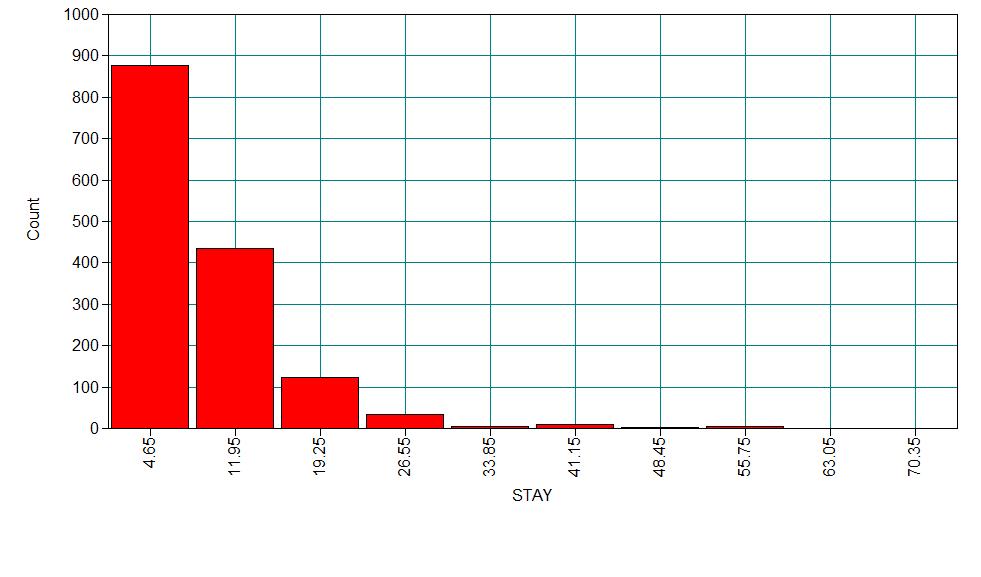
The variable describing length of hospital visit is stay
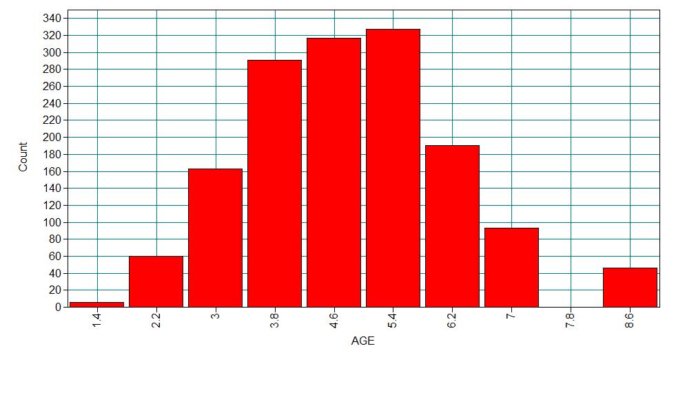
The variable age gives the age group from 1 to 9 which will be treated as
interval in this example.
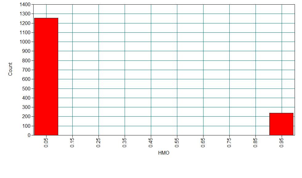
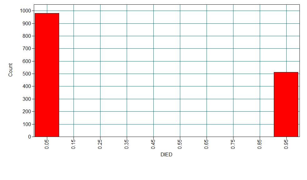
The variables hmo and died are binary indicator variables for HMO
insured patients and patients who died while in hospital, respectively.
Let’s look at the data.
Data:
  File is C:ztnb.dat;
Variable:
  Names are
     stay age hmo died;
  Missing are all (-9999) ;
Analysis:
  Type = basic ;
Plot:
  Type = plot1;

     ESTIMATED SAMPLE STATISTICS


           Means
              STAY          AGE           HMO           DIED
              ________      ________      ________      ________
      1         9.729         5.234         0.160         0.343


           Covariances
              STAY          AGE           HMO           DIED
              ________      ________      ________      ________
 STAY          66.100
 AGE           -0.615         2.785
 HMO           -0.169        -0.006         0.134
 DIED          -0.447         0.121         0.000         0.225


           Correlations
              STAY          AGE           HMO           DIED
              ________      ________      ________      ________
 STAY           1.000
 AGE           -0.045         1.000
 HMO           -0.057        -0.010         1.000
 DIED          -0.116         0.152         0.000         1.000
Analysis methods you might consider
Before we show how you can analyze these data with a zero-truncated negative binomial analysis, let’s
consider some other methods that you might use.
- Zero-truncated Negative Binomial Regression – The focus of this web page.
- Zero-truncated Poisson Regression – Useful if there is no overdispersion
in the zero truncated variable. Currently, zero-truncated poisson models are
not possible in Mplus. - Negative Binomial Regression – Ordinary negative binomial regression will have difficulty
with zero-truncated data. It will try to predict zero counts even though there are
no zero values. - Poisson Regression – The same concerns as for negative binomial regression, namely,
ordinary poisson regression will have difficulty with
zero-truncated data. It will try to predict zero counts even though there are
no zero values. - OLS Regression – You could try to analyze these data using OLS regression. However, count
data are highly non-normal and are not well estimated by OLS regression.
Zero-trunacated negative binomial regression
In the syntax below, we have indicated that stay is a count
variable by using the count statement. The (nbt) option is
used to indicate 2 things: that we are modeling our count variable with a
negative binomial distribution, and that we are specifying a zero-truncated model.
Without the (t) option we would be estimating a negative
binomial model without
zero-truncation. Also, we do not need a usevariables statement
because
we are using all of the variables in the data set in the current model.
We have omitted the missing statement because we have no missing data in
this data set. The default estimation method is MLR – maximum likelihood
parameter estimates with standard errors and a chi-square test statistic that
are robust to non-normality and non-independence of observations. The MLR standard errors
are computed using a sandwich estimator. This is what we generally call robust
standard errors. To get the "regular" standard errors, we use the estimator
= ml on the analysis statement. (In the next example, we will
omit the analysis statement and obtain the robust standard errors.)
Our regression equations is specified in the model statement: we are predicting
length of stay using age, hmo status and whether the
patient died.
Data:
  File is C:ztnb.dat ;
Variable:
  Names = stay age hmo died;
  Count = stay(nbt);
Model:
  stay on age hmo died;

MODEL FIT INFORMATION

Number of Free Parameters                        5

Loglikelihood

          H0 Value                       -4755.280
          H0 Scaling Correction Factor       1.156
            for MLR

Information Criteria

          Akaike (AIC)                    9520.559
          Bayesian (BIC)                  9547.102
          Sample-Size Adjusted BIC        9531.218
            (n* = (n + 2) / 24)


MODEL RESULTS

                                                    Two-Tailed
                    Estimate       S.E.  Est./S.E.    P-Value

 STAY       ON
    AGE               -0.016      0.013     -1.194      0.233
    HMO               -0.147      0.057     -2.571      0.010
    DIED              -0.218      0.053     -4.142      0.000

 Intercepts
    STAY               2.408      0.075     32.039      0.000

 Dispersion
    STAY               0.566      0.037     15.316      0.000
In the MODEL FIT INFORMATION portion of the output, you will find the log
likelihood for the final model as well as a number of fit statistics. In the
MODEL RESULTS section of the output you will find the negative binomial
regression coefficients (estimates) for each of the variables, standard errors
and the ratio of the estimate to its standard error. This can be used as a
Z test, where values greater than 2 are considered to be statistically
significant. We see that hmo and died but not age are
significant predictors of stay. Thus, for example, for patients who
use HMO services compared to those who do not, the log count of days stayed is
about 0.147 less.
Now let’s rerun the model without the analysis: estimator = ml statement in order to obtain robust standard errors.
Data:
  File is C:ztnb.dat ;
Variable:
  Names = stay age hmo died;
  Missing = all (-9999) ;
  Count = stay(nbt);
Model:
  stay on age hmo died;
Analysis:
  estimator = ml;


MODEL RESULTS

                                                    Two-Tailed
                    Estimate       S.E.  Est./S.E.    P-Value

 STAY       ON
    AGE               -0.016      0.013     -1.197      0.231
    HMO               -0.147      0.059     -2.483      0.013
    DIED              -0.218      0.046     -4.718      0.000

 Intercepts
    STAY               2.408      0.072     33.457      0.000

 Dispersion
    STAY               0.566      0.031     18.132      0.000
Robust standard errors tend to be larger than "regular" standard errors,
though not always as we see for the variable age. The results
changed very little when using regular standard errors.
Things to consider
- Count data often use an exposure variable to indicate the number of times the event
could have happened. You can incorporate exposure into your model by using the exposure()
option. - It is not recommended that zero-truncated negative binomial models be applied to
small samples. What constitutes a small sample does not seem to be clearly defined
in the literature. - Pseudo-R-squared values differ from OLS R-squareds, please see
FAQ: What are
pseudo R-squareds? for a discussion on this issue.
References
- Long, J. Scott (1997). Regression Models for Categorical and Limited
Dependent Variables. Thousand Oaks, CA: Sage Publications. - Hilbe, J. M. (2007). Negative binomial regression. Cambridge, UK: Cambridge
University Press.