
This page briefly introduces linear mixed models LMMs as a method
for analyzing data that are non independent, multilevel/hierarchical,
longitudinal, or correlated. We focus on the general concepts and
interpretation of LMMS, with less time spent on the theory and
technical details.
Background
Linear mixed models are an extension of simple linear
models to allow both fixed and random effects, and are particularly
used when there is non independence in the data, such as arises from
a hierarchical structure. For example, students could
be sampled from within classrooms, or patients from within doctors.
When there are multiple levels, such as patients seen by the same
doctor, the variability in the outcome can be thought of as being
either within group or between group. Patient level observations are
not independent, as within a given doctor patients are more similar.
Units sampled at the highest level (in our example, doctors) are
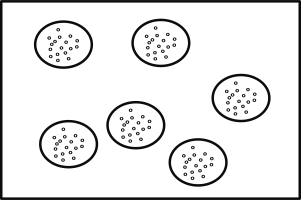
independent. The figure below shows a sample where the dots are patients
within doctors, the larger circles.
There are multiple ways to deal with hierarchical data.
One simple approach is to aggregate. For example, suppose
10 patients are sampled from each doctor. Rather than using the
individual patients’ data, which is not independent, we could
take the average of all patients within a doctor. This aggregated
data would then be independent.
Although aggregate data analysis yields consistent
effect estimates and standard errors, it does not really take
advantage of all the data, because patient data are simply
averaged. Looking at the figure above, at the aggregate level,
there would only be six data points.
Another approach to hierarchical data is analyzing data
from one unit at a time. Again in our example, we could run
six separate linear regressions—one for each doctor in the
sample. Again although this does work, there are many models,
and each one does not take advantage of the information
in data from other doctors. This can also make the results
“noisy” in that the estimates from each model are not based
on very much data
Linear mixed models (also called multilevel models) can
be thought of as a trade off between these two alternatives.
The individual regressions has many estimates and lots of data,
but is noisy. The aggregate is less noisy, but may lose important
differences by averaging all samples within each doctor. LMMs
are somewhere inbetween.
Beyond just caring about getting standard errors corrected
for non independence in the data, there can be important
reasons to explore the difference between effects within and
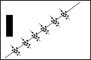
between groups. An example of this is shown in the figure
below. Here we have patients from the six doctors again,
and are looking at a scatter plot of the relation between
a predictor and outcome. Within each doctor, the relation
between predictor and outcome is negative. However, between
doctors, the relation is positive. LMMs allow us to explore
and understand these important effects.
Random Effects
The core of mixed models is that they incorporate
fixed and random effects. A fixed effect is a parameter
that does not vary. For example, we may assume there is
some true regression line in the population, \(\beta\),
and we get some estimate of it, \(\hat{\beta}\). In contrast,
random effects are parameters that are themselves random
variables. For example, we could say that \(\beta\) is
distributed as a random normal variate with mean \(\mu\) and
standard deviation \(\sigma\), or in equation form:
$$
\beta \sim \mathcal{N}(\mu, \sigma)
$$
This is really the same as in linear regression,
where we assume the data are random variables, but the
parameters are fixed effects. Now the data are random
variables, and the parameters are random variables
(at one level), but fixed at the highest level
(for example, we still assume some overall population mean,
\(\mu\) ).
Theory of Linear Mixed Models
$$
\mathbf{y} = \boldsymbol{X\beta} + \boldsymbol{Zu} + \boldsymbol{\varepsilon}
$$
Where \(\mathbf{y}\) is a \(N \times 1\) column vector, the outcome variable;
\(\mathbf{X}\) is a \(N \times p\) matrix of the \(p\) predictor variables;
\(\boldsymbol{\beta}\) is a \(p \times 1\) column vector of the fixed-effects regression
coefficients (the \(\beta\)s); \(\mathbf{Z}\) is the \(N \times qJ\) design matrix for
the \(q\) random effects and \(J\) groups;
\(\boldsymbol{u}\) is a \(qJ \times 1\) vector of \(q\) random
effects (the random complement to the fixed \(\boldsymbol{\beta})\) for \(J\) groups;
and \(\boldsymbol{\varepsilon}\) is a \(N \times 1\)
column vector of the residuals, that part of \(\mathbf{y}\) that is not explained by
the model, \(\boldsymbol{X\beta} + \boldsymbol{Zu}\). To recap:
$$
\overbrace{\mathbf{y}}^{\mbox{N x 1}} \quad = \quad
\overbrace{\underbrace{\mathbf{X}}_{\mbox{N x p}} \quad \underbrace{\boldsymbol{\beta}}_{\mbox{p x 1}}}^{\mbox{N x 1}} \quad + \quad
\overbrace{\underbrace{\mathbf{Z}}_{\mbox{N x qJ}} \quad \underbrace{\boldsymbol{u}}_{\mbox{qJ x 1}}}^{\mbox{N x 1}} \quad + \quad
\overbrace{\boldsymbol{\varepsilon}}^{\mbox{N x 1}}
$$
To make this more concrete, let’s consider an example from a
simulated dataset. Doctors (\(J = 407\)) indexed by the \(j\)
subscript each see \(n_{j}\) patients. So our grouping variable is the
doctor. Not every doctor sees the same number of patients, ranging
from just 2 patients all the way to 40 patients, averaging about
21. The total number of patients is the sum of the patients seen by
each doctor
$$
N = \sum_{j}^J n_j
$$
In our example, \(N = 8525\) patients were seen by doctors.
Our outcome, \(\mathbf{y}\) is a continuous variable,
mobility scores. Further, suppose we had 6 fixed effects predictors,
Age (in years), Married (0 = no, 1 = yes),
Sex (0 = female, 1 = male), Red Blood Cell (RBC) count, and
White Blood Cell (WBC) count plus a fixed intercept and
one random intercept ($q=1$) for each of the $J=407$ doctors. For simplicity, we are only going
to consider random intercepts. We will let every other effect be
fixed for now. The reason we want any random effects is because we
expect that mobility scores within doctors may be
correlated. There are many reasons why this could be. For example,
doctors may have specialties that mean they tend to see lung cancer
patients with particular symptoms or some doctors may see more
advanced cases, such that within a doctor,
patients are more homogeneous than they are between doctors.
To put this example back in our matrix notation, for the \(n_{j}\) dimensional response \(\mathbf{y_j}\) for doctor \(j\) we would have:
$$
\overbrace{\mathbf{y_j}}^{n_j \times 1} \quad = \quad
\overbrace{\underbrace{\mathbf{X_j}}_{n_j \times 6} \quad \underbrace{\boldsymbol{\beta}}_{6 \times 1}}^{n_j \times 1} \quad + \quad
\overbrace{\underbrace{\mathbf{Z_j}}_{n_j \times 1} \quad \underbrace{u_j}_{1 \times 1}}^{n_j \times 1} \quad + \quad
\overbrace{\boldsymbol{\varepsilon_j}}^{n_j \times 1}
$$
and by stacking observations from all groups together, since $q=1$ for the random intercept model, $qJ=(1)(407)=407$ so we have:
$$
\overbrace{\mathbf{y}}^{ 8525 \times 1} \quad = \quad
\overbrace{\underbrace{\mathbf{X}}_{ 8525 \times 6} \quad \underbrace{\boldsymbol{\beta}}_{6 \times 1}}^{ 8525 \times 1} \quad + \quad
\overbrace{\underbrace{\mathbf{Z}}_{ 8525 \times 407} \quad \underbrace{\boldsymbol{u}}_{ 407 \times 1}}^{ 8525 \times 1} \quad + \quad
\overbrace{\boldsymbol{\varepsilon}}^{ 8525 \times 1}
$$
$$
\mathbf{y} = \left[ \begin{array}{l} \text{mobility} \\ 2 \\ 2 \\ \ldots \\ 3 \end{array} \right] \begin{array}{l} n_{ij} \\ 1 \\ 2 \\ \ldots \\ 8525 \end{array} \quad \mathbf{X} = \left[ \begin{array}{llllll} \text{Intercept} & \text{Age} & \text{Married} & \text{Sex} & \text{WBC} & \text{RBC} \\ 1 & 64.97 & 0 & 1 & 6087 & 4.87 \\ 1 & 53.92 & 0 & 0 & 6700 & 4.68 \\ \ldots & \ldots & \ldots & \ldots & \ldots & \ldots \\ 1 & 56.07 & 0 & 1 & 6430 & 4.73 \\ \end{array} \right] $$
$$
\boldsymbol{\beta} =
\left[
\begin{array}{c}
4.782 \\
.025 \\
.011 \\
.012 \\
0 \\
-.009
\end{array}
\right]
$$
Because \(\mathbf{Z}\) is so big, we will not write out the numbers
here. Because we are only modeling random intercepts, it is a
special matrix in our case that only codes which doctor a patient
belongs to. So in this case, it is all 0s and 1s. Each column is one
doctor and each row represents one patient (one row in the
dataset). If the patient belongs to the doctor in that column, the
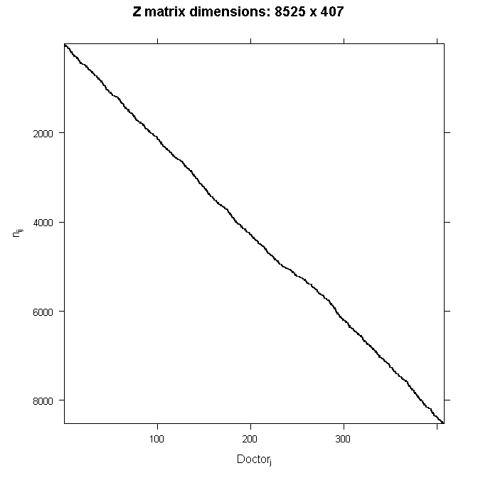
cell will have a 1, 0 otherwise. This also means that it is a sparse
matrix (i.e., a matrix of mostly zeros) and we can create a picture
representation easily. Note that if we added a random slope, the
number of rows in \(\mathbf{Z}\) would remain the same, but the
number of columns would double. This is why it can become
computationally burdensome to add random effects, particularly when
you have a lot of groups (we have 407 doctors). In all cases, the
matrix will contain mostly zeros, so it is always sparse. In the
graphical representation, the line appears to wiggle because the
number of patients per doctor varies.
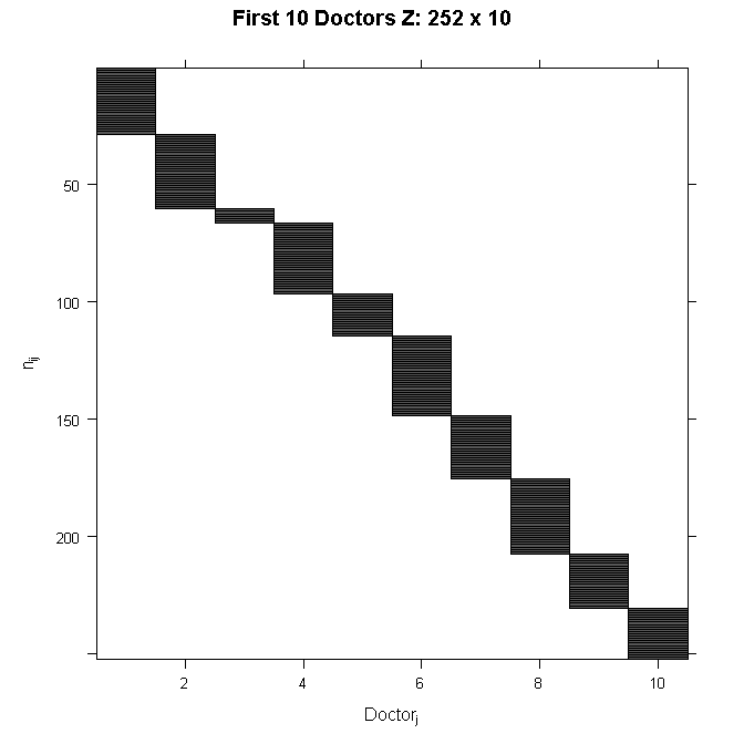
In order to see the structure in more detail, we could also zoom in
on just the first 10 doctors. The filled space indicates rows of
observations belonging to the doctor in that column, whereas the
white space indicates not belonging to the doctor in that column.
If we estimated it, \(\boldsymbol{u}\) would be a column
vector, similar to \(\boldsymbol{\beta}\). However, in classical
statistics, we do not actually estimate \(\boldsymbol{u}\).
Instead, we nearly always assume that:
$$
\boldsymbol{u} \sim \mathcal{N}(\mathbf{0}, \mathbf{G})
$$
Which is read: “\(\boldsymbol{u}\) is distributed as normal with mean zero and
variance \(\mathbf{G}\) “. Where \(\mathbf{G}\) is the variance-covariance matrix
of the random effects. Because we directly estimated the fixed
effects, including the fixed effect intercept, random effect
complements are modeled as deviations from the fixed effect, so they
have mean zero. The random effects are just deviations around the
value in \(\boldsymbol{\beta}\), which is the mean. So what is left
to estimate is the variance. Because our example only had a random
intercept, \(\mathbf{G}\) is just a \(1 \times 1\) matrix, the variance of
the random intercept (i.e. \(\mathbf{G}= [\sigma^{2}_{int}]\) ). However, it can be larger. For example,
suppose that we had a random intercept and a random slope, then
$$
\mathbf{G} =
\begin{bmatrix}
\sigma^{2}_{int} & \sigma^{2}_{int,slope} \\
\sigma^{2}_{int,slope} & \sigma^{2}_{slope}
\end{bmatrix}
$$
Because \(\mathbf{G}\) is a variance-covariance matrix, we know that
it should have certain properties. In particular, we know that it is
square, symmetric, and positive semidefinite. We also know that this matrix has
redundant elements. For a \(q \times q\) matrix, there are
\(\frac{q(q+1)}{2}\) unique elements. To simplify computation by
removing redundant effects and ensure that the resulting estimate
matrix is positive definite, rather than model \(\mathbf{G}\)
directly, we estimate \(\boldsymbol{\theta}\) (e.g., a triangular
Cholesky factorization \(\mathbf{G} = \mathbf{LDL^{T}}\)).
\(\boldsymbol{\theta}\) is not always parameterized the same way,
but you can generally think of it as representing the random
effects. It is usually designed to contain non redundant elements
(unlike the variance covariance matrix) and to be parameterized in a
way that yields more stable estimates than variances (such as taking
the natural logarithm to ensure that the variances are
positive). Regardless of the specifics, we can say that
$$
\mathbf{G} = \sigma(\boldsymbol{\theta})
$$
In other words, \(\mathbf{G}\) is some function of
\(\boldsymbol{\theta}\). So we get some estimate of
\(\boldsymbol{\theta}\) which we call \(\hat{\boldsymbol{\theta}}\).
Various parameterizations and constraints allow us to simplify the
model for example by assuming that the random effects are
independent, which would imply the true structure is
$$
\mathbf{G} =
\begin{bmatrix}
\sigma^{2}_{int} & 0 \\
0 & \sigma^{2}_{slope}
\end{bmatrix}
$$
The final element in our model is the variance-covariance matrix of the
residuals, \(\mathbf{\varepsilon}\) or the variance-covariance matrix of conditional distribution of
\((\mathbf{y} | \boldsymbol{\beta} ; \boldsymbol{u} = u)\).
The most common residual covariance structure is
$$
\mathbf{R} = \boldsymbol{I\sigma^2_{\varepsilon}}
$$
where \(\mathbf{I}\) is the identity matrix (diagonal matrix of 1s)
and \(\sigma^2_{\varepsilon}\) is the residual variance. This
structure assumes a homogeneous residual variance for all
(conditional) observations and that they are (conditionally)
independent. Other structures can be assumed such as compound
symmetry or autoregressive. The \(\mathbf{G}\) terminology is common
in SAS, and also leads to talking about G-side structures for the
variance covariance matrix of random effects and R-side structures
for the residual variance covariance matrix.
So the final fixed elements are \(\mathbf{y}\), \(\mathbf{X}\),
\(\mathbf{Z}\), and \(\boldsymbol{\varepsilon}\). The final estimated
elements are \(\hat{\boldsymbol{\beta}}\),
\(\hat{\boldsymbol{\theta}}\), and
\(\hat{\mathbf{R}}\). The final model depends on the distribution
assumed, but is generally of the form:
$$
(\mathbf{y} | \boldsymbol{\beta}; \boldsymbol{u} = u) \sim
\mathcal{N}(\boldsymbol{X\beta} + \boldsymbol{Z}u, \mathbf{R})
$$
We could also frame our model in a two level-style equation for
the \(i\)-th patient for the \(j\)-th doctor. There we are
working with variables that we subscript rather than vectors as
before. The level 1 equation adds subscripts to the parameters
\(\beta\)s to indicate which doctor they belong to. Turning to the
level 2 equations, we can see that each \(\beta\) estimate for a particular doctor,
\(\beta_{pj}\), can be represented as a combination of a mean estimate for that parameter, \(\gamma_{p0}\), and a random effect for that doctor, (\(u_{pj}\)).
In this particular model, we see that only the intercept
(\(\beta_{0j}\)) is allowed to vary across doctors because it is the only equation
with a random effect term, (\(u_{0j}\)). The other \(\beta_{pj}\) are constant across doctors.
$$
\begin{array}{l l}
L1: & Y_{ij} = \beta_{0j} + \beta_{1j}Age_{ij} + \beta_{2j}Married_{ij} + \beta_{3j}Sex_{ij} + \beta_{4j}WBC_{ij} + \beta_{5j}RBC_{ij} + e_{ij} \\
L2: & \beta_{0j} = \gamma_{00} + u_{0j} \\
L2: & \beta_{1j} = \gamma_{10} \\
L2: & \beta_{2j} = \gamma_{20} \\
L2: & \beta_{3j} = \gamma_{30} \\
L2: & \beta_{4j} = \gamma_{40} \\
L2: & \beta_{5j} = \gamma_{50}
\end{array}
$$
Substituting in the level 2 equations into level 1, yields the
mixed model specification. Here we grouped the fixed and random
intercept parameters together to show that combined they give the
estimated intercept for a particular doctor.
$$
Y_{ij} = (\gamma_{00} + u_{0j}) + \gamma_{10}Age_{ij} + \gamma_{20}Married_{ij} + \gamma_{30}SEX_{ij} + \gamma_{40}WBC_{ij} + \gamma_{50}RBC_{ij} + e_{ij}
$$
References
- Fox, J. (2008). Applied Regression Analysis and
Generalized Linear Models, 2nd ed. Sage Publications. - McCullagh, P, & Nelder, J. A. (1989). Generalized Linear
Models, 2nd ed. Chapman & Hall/CRC Press. - Snijders, T. A. B. & Bosker, R. J. (2012). Multilevel
Analysis, 2nd ed. Sage Publications. - Singer, J. D. & Willett, J. B. (2003). Applied
Longitudinal Data Analysis: Modeling Change and Event
Occurrence. Oxford University Press. - Pinheiro, J. & Bates, D. (2009). Mixed-Effects Models in
S and S-Plus. 2nd printing. Springer. - Galecki, A. & Burzykowski, T. (2013). Linear Mixed-Effects
Models Using R. Springer. - Skrondal, A. & Rabe-Hesketh, S. (2004). Generalized
Latent Variable Modeling: Multilevel, longitudinal, and structural
equation models. Chapman & Hall/CRC Press. - Gelman, A. & Hill, J. (2006). Data Analysis Using Regression
and Multilevel/Hierarchical Models. Cambridge University Press. - Gelman, A., Carlin, J. B., Stern, H. S. & Rubin, D. B. (2003).
Bayesian Data Analysis, 2nd ed. Chapman & Hall/CRC.