
Mixed effects cox regression models are used to model survival data
when there are repeated measures on an individual, individuals
nested within some other hierarchy, or some other reason to have both
fixed and random effects.
This page uses the following packages. Make sure that you can load
them before trying to run the examples on this page. If you do not have
a package installed, run: install.packages("packagename"), or
if you see the version is out of date, run: update.packages().
require(survival)
require(coxme)
Version info: Code for this page was tested in R version 3.0.1 (2013-05-16)

 On: 2013-06-26

With: coxme 2.2-3; Matrix 1.0-12; lattice 0.20-15; nlme 3.1-109; bdsmatrix 1.3-1; survival 2.37-4; knitr 1.2
Please note: The purpose of this page is to show how to use various
data analysis commands. It does not cover all aspects of the research process
which researchers are expected to do. In particular, it does not cover data
cleaning and checking, verification of assumptions, model diagnostics or
potential follow-up analyses.
Examples of mixed effects cox models
Example 1.
Example 2.
Description of the data
########## simulate data ##########
set.seed(10)
N <- 250
dat <- data.frame(ID = factor(1:N), age = rnorm(N, mean = 45, sd = 5), sex = sample(0:1,
    N, TRUE), basemort = rnorm(N, sd = 3))

interval <- matrix(sample(2:14, N * 3, replace = TRUE), N)
windows <- t(apply(cbind(0, interval), 1, cumsum))
windows <- rbind(windows[, 1:2], windows[, 2:3], windows[, 3:4])

colnames(windows) <- c("time1", "time2")
dat <- cbind(do.call(rbind, rep(list(dat), 3)), windows)
dat <- dat[order(dat$ID), ]
dat$assessment <- rep(1:3, N)
rownames(dat) <- NULL
head(dat)
##   ID  age sex basemort time1 time2 assessment
## 1  1 45.1   1    6.659     0    14          1
## 2  1 45.1   1    6.659    14    16          2
## 3  1 45.1   1    6.659    16    23          3
## 4  2 44.1   1    0.943     0     8          1
## 5  2 44.1   1    0.943     8    20          2
## 6  2 44.1   1    0.943    20    22          3
# simulate survival (mortality) data
transplant <- with(dat, {
    mu <- (0.05 * age) + (0.3 * time2)
    lp <- rnorm(N * 3, mean = mu, sd = 1)
    as.integer(lp > quantile(lp, probs = 0.65))
})
# ensure that transplants do not revert
transplant <- as.integer(ave(transplant, dat$ID, FUN = cumsum) >= 1)

# simulate survival (mortality) data
mortality <- with(dat, {
    mu <- basemort + (0.05 * age) - (2.5 * sex) + (0.3 * time2)
    lp <- rnorm(N * 3, mean = mu, sd = 1)
    as.integer(lp > median(lp))
})

# ensure that once someone dies, he or she stays dead
mortality <- as.integer(ave(mortality, dat$ID, FUN = cumsum) >= 1)

# ensure no one dead at baseline
mortality[dat$assessment == 1] <- 0

# ensure no post mortem change in transplant status
transplant <- unlist(by(data.frame(mortality, transplant), dat$ID, FUN = function(x) {
    i <- cumsum(x$mortality)
    tstat <- x$transplant[i == 1]
    x$transplant[i >= 1] <- tstat
    return(x$transplant)
}))

dat$transplant <- transplant
dat$mortality <- mortality

# print first few rows
head(dat)
##   ID  age sex basemort time1 time2 assessment transplant mortality
## 1  1 45.1   1    6.659     0    14          1          0         0
## 2  1 45.1   1    6.659    14    16          2          0         1
## 3  1 45.1   1    6.659    16    23          3          0         1
## 4  2 44.1   1    0.943     0     8          1          0         0
## 5  2 44.1   1    0.943     8    20          2          1         1
## 6  2 44.1   1    0.943    20    22          3          1         1
Analysis methods you might consider
- Cox regression, does not account for random effects.
- Mixed effects cox regression, the focus of this page.
- Logistic regression, does not account for the baseline
hazard or mixed effects. - Mixed effects logistic regression, does not account for
the baseline hazard.
Mixed effects cox regression
########## basic models ########## simple model
m <- coxph(Surv(time1, time2, mortality) ~ age + sex + transplant, data = dat)
## summary of the model
summary(m)
## Call:
## coxph(formula = Surv(time1, time2, mortality) ~ age + sex + transplant,
##     data = dat)
##
##   n= 750, number of events= 313
##
##               coef exp(coef) se(coef)     z Pr(>|z|)
## age        -0.0124    0.9876   0.0128 -0.97    0.333
## sex        -0.2899    0.7483   0.1160 -2.50    0.012 *
## transplant -0.8505    0.4272   0.1253 -6.79  1.1e-11 ***
## ---
## Signif. codes:  0 '***' 0.001 '**' 0.01 '*' 0.05 '.' 0.1 ' ' 1
##
##            exp(coef) exp(-coef) lower .95 upper .95
## age            0.988       1.01     0.963     1.013
## sex            0.748       1.34     0.596     0.939
## transplant     0.427       2.34     0.334     0.546
##
## Concordance= 0.66  (se = 0.02 )
## Rsquare= 0.076   (max possible= 0.98 )
## Likelihood ratio test= 59.5  on 3 df,   p=7.48e-13
## Wald test            = 61.2  on 3 df,   p=3.25e-13
## Score (logrank) test = 63.6  on 3 df,   p=9.91e-14
## model with robust SE via clustering
m2 <- coxph(Surv(time1, time2, mortality) ~ age + sex + transplant + cluster(ID),
    data = dat)
## summary of the model
summary(m2)
## Call:
## coxph(formula = Surv(time1, time2, mortality) ~ age + sex + transplant +
##     cluster(ID), data = dat)
##
##   n= 750, number of events= 313
##
##               coef exp(coef) se(coef) robust se     z Pr(>|z|)
## age        -0.0124    0.9876   0.0128    0.0131 -0.95   0.3415
## sex        -0.2899    0.7483   0.1160    0.1122 -2.58   0.0098 **
## transplant -0.8505    0.4272   0.1253    0.1218 -6.98  2.9e-12 ***
## ---
## Signif. codes:  0 '***' 0.001 '**' 0.01 '*' 0.05 '.' 0.1 ' ' 1
##
##            exp(coef) exp(-coef) lower .95 upper .95
## age            0.988       1.01     0.963     1.013
## sex            0.748       1.34     0.601     0.932
## transplant     0.427       2.34     0.336     0.542
##
## Concordance= 0.66  (se = 0.02 )
## Rsquare= 0.076   (max possible= 0.98 )
## Likelihood ratio test= 59.5  on 3 df,   p=7.48e-13
## Wald test            = 58.6  on 3 df,   p=1.17e-12
## Score (logrank) test = 63.6  on 3 df,   p=9.91e-14,   Robust = 67.6  p=1.39e-14
##
##   (Note: the likelihood ratio and score tests assume independence of
##      observations within a cluster, the Wald and robust score tests do not).
## model with a frailty term (slower)
m3 <- coxph(Surv(time1, time2, mortality) ~ age + sex + transplant + frailty(ID,
    distribution = "gaussian", sparse = FALSE, method = "reml"), data = dat)
## show model results
m3
## Call:
## coxph(formula = Surv(time1, time2, mortality) ~ age + sex + transplant +
##     frailty(ID, distribution = "gaussian", sparse = FALSE, method = "reml"),
##     data = dat)
##
##                           coef   se(coef) se2    Chisq DF  p
## age                       -0.013 0.0132   0.0129  0.97 1.0 3.3e-01
## sex                       -0.301 0.1196   0.1160  6.31 1.0 1.2e-02
## transplant                -0.881 0.1301   0.1260 45.81 1.0 1.3e-11
## frailty(ID, distribution                          9.98 9.5 4.0e-01
##
## Iterations: 8 outer, 23 Newton-Raphson
##      Variance of random effect= 0.0338
## Degrees of freedom for terms= 0.9 0.9 0.9 9.5
## Likelihood ratio test=538  on 12.3 df, p=0  n= 750
########## cox model with random effects ########## given repeated
########## observations on individuals each individual likely has their
########## own baseline so adjust with a mixed effects cox model using
########## the coxme package

m4 <- coxme(Surv(time1, time2, mortality) ~ age + sex + transplant + (1 |
    ID), data = dat)
## just print, no summary
m4
## Cox mixed-effects model fit by maximum likelihood
##   Data: dat
##   events, n = 313, 750
##   Iterations= 10 43
##                 NULL Integrated Fitted
## Log-likelihood -1474      -1445  -1440
##
##                   Chisq   df        p  AIC  BIC
## Integrated loglik  59.6 4.00 3.60e-12 51.6 36.6
##  Penalized loglik  68.7 7.43 4.64e-12 53.8 26.0
##
## Model:  Surv(time1, time2, mortality) ~ age + sex + transplant + (1 |      ID)
## Fixed coefficients
##               coef exp(coef) se(coef)     z       p
## age        -0.0127     0.987    0.013 -0.97 3.3e-01
## sex        -0.2949     0.745    0.118 -2.51 1.2e-02
## transplant -0.8652     0.421    0.128 -6.78 1.2e-11
##
## Random effects
##  Group Variable  Std Dev Variance
##  ID    Intercept 0.1234  0.0152
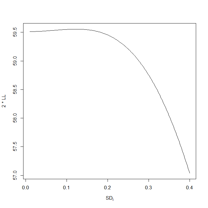
## Get profile likelihood for variance values to examine, based on
## observed .486
s <- seq(0.01, 0.4, length.out = 200)^2
res <- sapply(s, function(i) {
    mod <- coxme(Surv(time1, time2, mortality) ~ age + sex + transplant +
        (1 | ID), data = dat, vfixed = i)
    2 * diff(mod$loglik)[1]
})

## profile likelihood, horizontal line is 95% CI obviously lower bound
## includes 0, upper bound looks a little under .8

plot(sqrt(s), res, type = "l", xlab = expression(SD[i]), ylab = "2 * LL")
abline(h = 2 * diff(m4$loglik)[1] - qchisq(0.95, 1), lty = 2)
## compare models
summary(m)  # regular cox no adjust for repeated measures
## Call:
## coxph(formula = Surv(time1, time2, mortality) ~ age + sex + transplant,
##     data = dat)
##
##   n= 750, number of events= 313
##
##               coef exp(coef) se(coef)     z Pr(>|z|)
## age        -0.0124    0.9876   0.0128 -0.97    0.333
## sex        -0.2899    0.7483   0.1160 -2.50    0.012 *
## transplant -0.8505    0.4272   0.1253 -6.79  1.1e-11 ***
## ---
## Signif. codes:  0 '***' 0.001 '**' 0.01 '*' 0.05 '.' 0.1 ' ' 1
##
##            exp(coef) exp(-coef) lower .95 upper .95
## age            0.988       1.01     0.963     1.013
## sex            0.748       1.34     0.596     0.939
## transplant     0.427       2.34     0.334     0.546
##
## Concordance= 0.66  (se = 0.02 )
## Rsquare= 0.076   (max possible= 0.98 )
## Likelihood ratio test= 59.5  on 3 df,   p=7.48e-13
## Wald test            = 61.2  on 3 df,   p=3.25e-13
## Score (logrank) test = 63.6  on 3 df,   p=9.91e-14
m4 # cox with mixed effects
## Cox mixed-effects model fit by maximum likelihood
##   Data: dat
##   events, n = 313, 750
##   Iterations= 10 43
##                 NULL Integrated Fitted
## Log-likelihood -1474      -1445  -1440
##
##                   Chisq   df        p  AIC  BIC
## Integrated loglik  59.6 4.00 3.60e-12 51.6 36.6
##  Penalized loglik  68.7 7.43 4.64e-12 53.8 26.0
##
## Model:  Surv(time1, time2, mortality) ~ age + sex + transplant + (1 |      ID)
## Fixed coefficients
##               coef exp(coef) se(coef)     z       p
## age        -0.0127     0.987    0.013 -0.97 3.3e-01
## sex        -0.2949     0.745    0.118 -2.51 1.2e-02
## transplant -0.8652     0.421    0.128 -6.78 1.2e-11
##
## Random effects
##  Group Variable  Std Dev Variance
##  ID    Intercept 0.1234  0.0152
########################################################
Things to consider
See also