
Poisson regression is used to model count variables.
This page uses the following packages. Make sure that you can load
them before trying to run the examples on this page. If you do not have
a package installed, run: install.packages("packagename"), or
if you see the version is out of date, run: update.packages().
require(ggplot2)
require(sandwich)
require(msm)
Version info: Code for this page was tested in R version 3.1.1 (2014-07-10)

On: 2014-08-11

With: sandwich 2.3-1; boot 1.3-11; knitr 1.6; pscl 1.04.4; vcd 1.3-1; gam 1.09.1; coda 0.16-1; mvtnorm 1.0-0; GGally 0.4.7; plyr 1.8.1; MASS 7.3-33; Hmisc 3.14-4; Formula 1.1-2; survival 2.37-7; psych 1.4.5; reshape2 1.4; msm 1.4; phia 0.1-5; RColorBrewer 1.0-5; effects 3.0-0; colorspace 1.2-4; lattice 0.20-29; pequod 0.0-3; car 2.0-20; ggplot2 1.0.0
Please note: The purpose of this page is to show how to use various data
analysis commands. It does not cover all aspects of the research process which
researchers are expected to do. In particular, it does not cover data
cleaning and checking, verification of assumptions, model diagnostics or
potential follow-up analyses.
Examples of Poisson regression
Example 1. The number of persons killed by mule or horse kicks in the
Prussian army per year. Ladislaus Bortkiewicz collected data from 20 volumes of
Preussischen Statistik. These data were collected on 10 corps of
the Prussian army in the late 1800s over the course of 20 years.
Example 2. The number of people in line in front of you at the grocery store.
Predictors may include the number of items currently offered at a special
discounted price and whether a special event (e.g., a holiday, a big sporting
event) is three or fewer days away.
Example 3. The number of awards earned by students at one high school.
Predictors of the number of awards earned include the type of program in which the
student was enrolled (e.g., vocational, general or academic) and the score on their
final exam in math.
Description of the data
For the purpose of illustration, we have simulated a data set for Example 3 above.
In this example, num_awards is the outcome variable and indicates the
number of awards earned by students at a high school in a year, math is a continuous
predictor variable and represents students’ scores on their math final exam, and prog is a categorical predictor variable with
three levels indicating the type of program in which the students were
enrolled. It is coded as 1 = “General”, 2 = “Academic” and 3 = “Vocational”.
Let’s start with loading the data and looking at some descriptive statistics.
p <- read.csv("https://stats.idre.ucla.edu/stat/data/poisson_sim.csv")
p <- within(p, {
  prog <- factor(prog, levels=1:3, labels=c("General", "Academic",
                                                     "Vocational"))
  id <- factor(id)
})
summary(p)
##        id        num_awards           prog          math
##  1      :  1   Min.   :0.00   General   : 45   Min.   :33.0
##  2      :  1   1st Qu.:0.00   Academic  :105   1st Qu.:45.0
##  3      :  1   Median :0.00   Vocational: 50   Median :52.0
##  4      :  1   Mean   :0.63                    Mean   :52.6
##  5      :  1   3rd Qu.:1.00                    3rd Qu.:59.0
##  6      :  1   Max.   :6.00                    Max.   :75.0
##  (Other):194
Each variable has 200 valid observations and their distributions seem quite
reasonable. The unconditional mean and variance of our outcome variable
are not extremely different. Our model assumes that these values, conditioned on
the predictor variables, will be equal (or at least roughly so).
We can use the tapply function to display the summary statistics by program
type. The table below shows the average numbers of awards by program type
and seems to suggest that program type is a good candidate for
predicting the number of awards, our outcome variable, because the mean value of
the outcome appears to vary by prog. Additionally, the
means and variances within each level of prog–the conditional
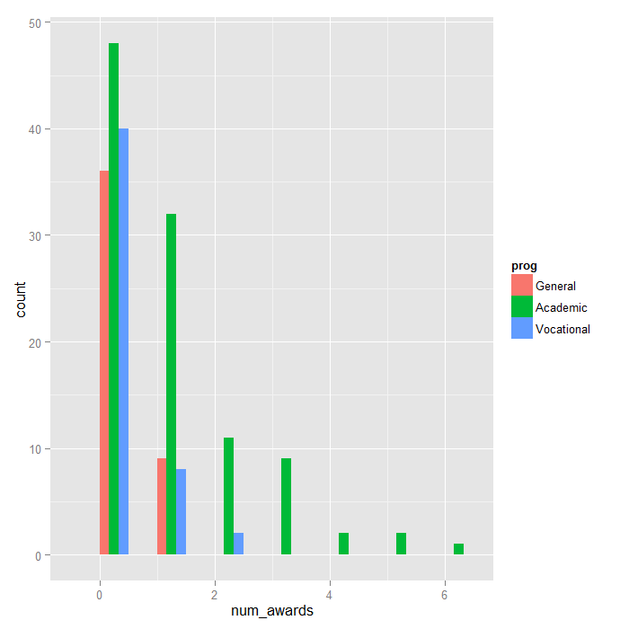
means and variances–are similar. A conditional histogram separated out by
program type is plotted to show the distribution.
with(p, tapply(num_awards, prog, function(x) {
  sprintf("M (SD) = %1.2f (%1.2f)", mean(x), sd(x))
}))
##                General               Academic             Vocational
## "M (SD) = 0.20 (0.40)" "M (SD) = 1.00 (1.28)" "M (SD) = 0.24 (0.52)"
ggplot(p, aes(num_awards, fill = prog)) +
  geom_histogram(binwidth=.5, position="dodge")
Analysis methods you might consider
Below is a list of some analysis methods you may have
encountered. Some of the methods listed are quite reasonable, while others have
either fallen out of favor or have limitations.
- Poisson regression – Poisson regression is often used for modeling count
data. Poisson regression has a number of extensions useful for count models. - Negative binomial regression – Negative binomial regression can be used for over-dispersed
count data, that is when the conditional variance exceeds the conditional
mean. It can be considered as a generalization of Poisson regression since
it has the same mean structure as Poisson regression and it has an extra
parameter to model the over-dispersion. If the conditional distribution of
the outcome variable is over-dispersed, the confidence intervals for coefficients in Negative binomial
regression are likely to be wider as compared to those from a Poisson regression. - Zero-inflated regression model – Zero-inflated models attempt to account
for excess zeros. In other words, two kinds of zeros are thought to
exist in the data, “true zeros” and “excess zeros”. Zero-inflated
models estimate two equations simultaneously, one for the count model and one for the
excess zeros. - OLS regression – Count outcome variables are sometimes log-transformed
and analyzed using OLS regression. Many issues arise with this
approach, including loss of data due to undefined values generated by taking
the log of zero (which is undefined) and biased estimates.
Poisson regression
At this point, we are ready to perform our Poisson model analysis using
the glm function. We fit the model and store it in the object m1
and get a summary of the model at the same time.
summary(m1 <- glm(num_awards ~ prog + math, family="poisson", data=p))
##
## Call:
## glm(formula = num_awards ~ prog + math, family = "poisson", data = p)
##
## Deviance Residuals:
##    Min      1Q  Median      3Q     Max
## -2.204  -0.844  -0.511   0.256   2.680
##
## Coefficients:
##                Estimate Std. Error z value Pr(>|z|)
## (Intercept)     -5.2471     0.6585   -7.97  1.6e-15 ***
## progAcademic     1.0839     0.3583    3.03   0.0025 **
## progVocational   0.3698     0.4411    0.84   0.4018
## math             0.0702     0.0106    6.62  3.6e-11 ***
## ---
## Signif. codes:  0 '***' 0.001 '**' 0.01 '*' 0.05 '.' 0.1 ' ' 1
##
## (Dispersion parameter for poisson family taken to be 1)
##
##     Null deviance: 287.67  on 199  degrees of freedom
## Residual deviance: 189.45  on 196  degrees of freedom
## AIC: 373.5
##
## Number of Fisher Scoring iterations: 6
Cameron and Trivedi (2009) recommended using robust standard errors for the
parameter estimates to control for mild violation of the distribution
assumption that the variance equals the mean.
We use R package sandwich below to obtain the robust standard errors and
calculated the p-values accordingly. Together with the p-values, we have also
calculated the 95% confidence interval using the parameter estimates and their
robust standard errors.
cov.m1 <- vcovHC(m1, type="HC0")
std.err <- sqrt(diag(cov.m1))
r.est <- cbind(Estimate= coef(m1), "Robust SE" = std.err,
"Pr(>|z|)" = 2 * pnorm(abs(coef(m1)/std.err), lower.tail=FALSE),
LL = coef(m1) - 1.96 * std.err,
UL = coef(m1) + 1.96 * std.err)

r.est
##                Estimate Robust SE  Pr(>|z|)      LL       UL
## (Intercept)    -5.24712   0.64600 4.567e-16 -6.5133 -3.98097
## progAcademic    1.08386   0.32105 7.355e-04  0.4546  1.71311
## progVocational  0.36981   0.40042 3.557e-01 -0.4150  1.15463
## math            0.07015   0.01044 1.784e-11  0.0497  0.09061
Now let’s look at the output of function glm more closely.
- The output begins
with echoing the function call. The information on deviance residuals
is displayed next. Deviance residuals are approximately normally distributed
if the model is specified correctly.In our example, it shows a little
bit of skeweness since median is not quite zero. - Next come the Poisson regression coefficients for each of the variables
along with the standard errors, z-scores, p-values
and 95% confidence intervals for the coefficients. The coefficient for
mathis .07. This means that the expected
log count for a one-unit increase inmathis .07. The indicator variable
progAcademiccompares between prog = “Academic”
and prog = “General”, the expected log count for prog =
“Academic” increases by about 1.1. The
indicator variableprog.Vocationalis the expected
difference in log count ((approx .37)) between prog = “Vocational” and
the reference group (prog = “General”). - The information on deviance is also provided. We can use the residual
deviance to perform a goodness of fit test for the overall model. The
residual deviance is the difference between the deviance of the current
model and the maximum deviance of the ideal model where the predicted values
are identical to the observed. Therefore, if the residual difference is
small enough, the goodness of fit test will not be significant, indicating
that the model fits the data. We conclude that the model fits reasonably
well because the goodness-of-fit chi-squared test is not statistically
significant. If the test had been statistically significant, it would
indicate that the data do not fit the model well. In that situation,
we may try to determine if there are omitted predictor variables, if
our linearity assumption holds and/or if there is an issue of
over-dispersion.
with(m1, cbind(res.deviance = deviance, df = df.residual,
  p = pchisq(deviance, df.residual, lower.tail=FALSE)))
##      res.deviance  df      p
## [1,]        189.4 196 0.6182
We can also test the overall effect of prog by comparing the deviance
of the full model with the deviance of the model excluding prog.
The two degree-of-freedom chi-square test indicates that prog, taken
together, is a statistically significant predictor of num_awards.
## update m1 model dropping prog
m2 <- update(m1, . ~ . - prog)
## test model differences with chi square test
anova(m2, m1, test="Chisq")
## Analysis of Deviance Table
##
## Model 1: num_awards ~ math
## Model 2: num_awards ~ prog + math
##   Resid. Df Resid. Dev Df Deviance Pr(>Chi)
## 1       198        204
## 2       196        189  2     14.6  0.00069 ***
## ---
## Signif. codes:  0 '***' 0.001 '**' 0.01 '*' 0.05 '.' 0.1 ' ' 1
Sometimes, we might want to present the regression results as incident rate
ratios and their standard errors, together with the confidence interval. To
compute the standard error for the incident rate ratios, we will use the
Delta method. To this end, we make use the function deltamethod
implemented in R package msm.
s <- deltamethod(list(~ exp(x1), ~ exp(x2), ~ exp(x3), ~ exp(x4)),
                                                coef(m1), cov.m1)

## exponentiate old estimates dropping the p values
rexp.est <- exp(r.est[, -3])
## replace SEs with estimates for exponentiated coefficients
rexp.est[, "Robust SE"] <- s

rexp.est
##                Estimate Robust SE       LL      UL
## (Intercept)    0.005263   0.00340 0.001484 0.01867
## progAcademic   2.956065   0.94904 1.575551 5.54620
## progVocational 1.447458   0.57959 0.660335 3.17284
## math           1.072672   0.01119 1.050955 1.09484
The output above indicates that the incident rate for prog = “Academic” is 2.96
times the incident rate for the reference group (prog = “General”). Likewise,
the incident rate for prog = “Vocational” is 1.45 times the incident rate for the
reference group holding the other variables at constant. The percent change in the incident rate of
num_awards is by 7% for every unit increase in math.
For additional information on the various metrics in which the results can be
presented, and the interpretation of such, please see Regression Models for
Categorical Dependent Variables Using Stata, Second Edition by J. Scott Long
and Jeremy Freese (2006).
Sometimes, we might want to look at the expected marginal means. For
example, what are the expected counts for each program type holding math
score at its overall mean? To answer this question, we can make use of
the predict function. First off, we will make a small data set
to apply the predict function to it.
(s1 <- data.frame(math = mean(p$math),
  prog = factor(1:3, levels = 1:3, labels = levels(p$prog))))
##    math       prog
## 1 52.65    General
## 2 52.65   Academic
## 3 52.65 Vocational
predict(m1, s1, type="response", se.fit=TRUE)
## $fit
##      1      2      3
## 0.2114 0.6249 0.3060
##
## $se.fit
##       1       2       3
## 0.07050 0.08628 0.08834
##
## $residual.scale
## [1] 1
In the output above, we see that the predicted number of events for level 1
of prog is about .21, holding math at its mean. The predicted
number of events for level 2 of prog is higher at .62, and the
predicted number of events for level 3 of prog is about .31. The ratios
of these predicted counts ((frac{.625}{.211} = 2.96), (frac{.306}{.211} = 1.45)) match
what we saw looking at the IRR.
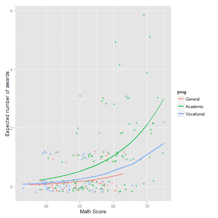
We can also graph the predicted number of events with the commands below.
The graph indicates that the most awards are predicted for those in the academic
program (prog = 2), especially if the student has a high math score. The
lowest number of predicted awards is for those students in the general program (prog
= 1). The graph overlays the lines of expected values onto the actual points,
although a small amount of random noise was added vertically to lessen
overplotting.
## calculate and store predicted values
p$phat <- predict(m1, type="response")

## order by program and then by math
p <- p[with(p, order(prog, math)), ]

## create the plot
ggplot(p, aes(x = math, y = phat, colour = prog)) +
  geom_point(aes(y = num_awards), alpha=.5, position=position_jitter(h=.2)) +
  geom_line(size = 1) +
  labs(x = "Math Score", y = "Expected number of awards")
Things to consider
- When there seems to be an issue of dispersion, we should first check if
our model is appropriately specified, such as omitted variables and
functional forms. For example, if we omitted the predictor variableprogin the example above, our model would seem to have a problem with
over-dispersion. In other words, a misspecified model could present
a symptom like an over-dispersion problem. - Assuming that the model is correctly specified, the assumption that the
conditional variance is equal to the conditional mean should be checked.
There are several tests including the likelihood ratio test of
over-dispersion parameter alpha by running the same model using negative
binomial distribution. R package
pscl (Political Science Computational Laboratory, Stanford University)
provides many functions for binomial and count data includingodTest
for testing over-dispersion. - One common cause of over-dispersion is excess zeros, which in turn are
generated by an additional data generating process. In this situation,
zero-inflated model should be considered. - If the data generating process does not allow for any 0s (such as the
number of days spent in the hospital), then a zero-truncated model may be
more appropriate. - Count data often have an exposure variable, which indicates the number
of times the event could have happened. This variable should be
incorporated into a Poisson model with the use of theoffsetoption. - The outcome variable in a Poisson regression cannot have negative numbers, and the exposure
cannot have 0s. - Many different measures of pseudo-R-squared exist.
They all attempt to provide information similar to that provided by
R-squared in OLS regression, even though none of them can be interpreted
exactly as R-squared in OLS regression is interpreted. For a discussion of
various pseudo-R-squares, see Long and Freese (2006) or our FAQ page
What are pseudo R-squareds?. - Poisson regression is estimated via maximum likelihood estimation. It
usually requires a large sample size.
References
- Cameron, A. C. and Trivedi, P. K. 2009. Microeconometrics Using
Stata. College Station, TX: Stata Press. - Cameron, A. C. and Trivedi, P. K. 1998. Regression
Analysis of Count Data. New York: Cambridge Press. - Cameron, A. C. Advances in Count Data Regression Talk for the
Applied Statistics Workshop, March 28, 2009.
http://cameron.econ.ucdavis.edu/racd/count.html . - Dupont, W. D. 2002. Statistical Modeling for Biomedical
Researchers: A Simple Introduction to the Analysis of Complex Data.
New York: Cambridge Press. - Long, J. S. 1997. Regression Models for Categorical and Limited Dependent Variables.
Thousand Oaks, CA: Sage Publications. - Long, J. S. and Freese, J. 2006. Regression Models for
Categorical Dependent Variables Using Stata, Second Edition.
College Station, TX: Stata Press.