
Choose the software whose output you would like to interpret.
This page shows an example of logit regression with footnotes explaining the output. First an example is shown using Stata, and then an example is shown using Mplus, to help you relate the output you are likely to be familiar with (Stata) to output that may be new to you (Mplus). We suggest that you view this page using two web browsers so you can show the page side by side showing the Stata output in one browser and the corresponding Mplus output in the other browser.
This example is from the Mplus User’s Guide (example 3.5) and we suggest that you see the Mplus User’s Guide for more details about this example. We thank the kind people at Muthén & Muthén for permission to use examples from their manual.
Example Using Stata
Here is a logit regression example using Stata with two continuous predictors x1 and x2 used to predict a binary outcome variable, u1.
infile u1 x1 x3 using https://stats.idre.ucla.edu/wp-content/uploads/2016/02/ex3.5.dat, clear
tabulate u1

         u1 |      Freq.     Percent        Cum.
------------+-----------------------------------
          0 |        327       65.40A       65.40
          1 |        173       34.60A      100.00
------------+-----------------------------------
      Total |        500      100.00
A. These are the percent of cases with 0 and 1 on the variable u1
logit u1 x1 x3

Iteration 0:   log likelihood = -322.46763
Iteration 1:   log likelihood = -216.57883
Iteration 2:   log likelihood = -203.79479
Iteration 3:   log likelihood = -202.63515
Iteration 4:   log likelihood = -202.61995
Iteration 5:   log likelihood = -202.61995

Logistic regression                               Number of obs   =        500
                                                  LR chi2(2)      =     239.70
                                                  Prob > chi2     =     0.0000
Log likelihood = -202.61995                       Pseudo R2       =     0.3717

------------------------------------------------------------------------------
          u1 |      Coef.   Std. Err.      z    P>|z|     [95% Conf. Interval]
-------------+----------------------------------------------------------------
          x1 |   1.071767E  .1428573     7.50   0.000      .791772    1.351762
          x3 |   1.838588E  .1794923    10.24   0.000     1.486789    2.190386
       _cons |  -1.025842D  .1369173    -7.49   0.000    -1.294195   -.7574886
------------------------------------------------------------------------------
logit , or

Logistic regression                               Number of obs   =        500
                                                  LR chi2(2)      =     239.70
                                                  Prob > chi2     =     0.0000
Log likelihood = -202.61995                       Pseudo R2       =     0.3717

------------------------------------------------------------------------------
          u1 | Odds Ratio   Std. Err.      z    P>|z|     [95% Conf. Interval]
-------------+----------------------------------------------------------------
          x1 |   2.920536F   .4172198     7.50   0.000     2.207304    3.864229
          x3 |   6.287652F   1.128585    10.24   0.000     4.422872    8.938663
------------------------------------------------------------------------------
estat ic

------------------------------------------------------------------------------
       Model |    Obs    ll(null)   ll(model)B    df         AICC        BICC
-------------+----------------------------------------------------------------
           . |    500   -322.4676   -202.6199      3     411.2399    423.8837
------------------------------------------------------------------------------
The output is labeled with superscripts to help you relate the later Mplus output to this Stata output. To summarize the output, both predictors in this model, x1 and x2, are significantly related to the outcome variable, u1. The coefficients from the logit output can be exponentiated to obtain odds ratios, as shown in the output from the logit, or command. For a one unit increase in x1, the odds of u1 equaling 1 (as compared to u1 equaling 0) increases by a factor of 2.92. The estat ic command produces fit indices for the model including the log likelihood for the empty (null) model, the log likelihood for the model, as well as the AIC and BIC fit indices.
Mplus Example #1
Here is the same example illustrated in Mplus based on the https://stats.idre.ucla.edu/wp-content/uploads/2016/02/ex3.5.dat data file.
TITLE:
  this is an example of a logistic
  regression for a categorical observed
  dependent variable with two covariates
DATA:
  FILE = https://stats.idre.ucla.edu/wp-content/uploads/2016/02/ex3.5.dat;
VARIABLE:
  NAMES = u1 x1 x3;
  CATEGORICAL = u1;
ANALYSIS:
  ESTIMATOR = ML;
  ! need to use estimator = ml to make this a logistic model;
MODEL:
  u1 ON x1 x3;

SUMMARY OF ANALYSIS
Number of observations                                         500
Estimator                                                      MLR

<some output was omitted to save space>

SUMMARY OF CATEGORICAL DATA PROPORTIONS

    U1
      Category 1    0.654A
      Category 2    0.346A

TESTS OF MODEL FIT

Loglikelihood

          H0 Value                        -202.620B

Information Criteria

          Number of Free Parameters              3
          Akaike (AIC)                     411.240C
          Bayesian (BIC)                   423.884C
          Sample-Size Adjusted BIC         414.362
            (n* = (n + 2) / 24)
MODEL RESULTS

                   Estimates     S.E.  Est./S.E.

 U1         ON
    X1                 1.072D    0.143      7.502
    X3                 1.839D    0.179     10.243

 Thresholds
    U1$1               1.026E    0.137      7.492

LOGISTIC REGRESSION ODDS RATIO RESULTS

 U1         ON
    X1                 2.921F
    X3                 6.288F
- These are the percent of cases with 0 and 1 on the variable u1, see output of
tabulate command from Stata - This is the log likelihood value associated with the model (see the ll(model)
from the estat ic command in Stata. - These are the AIC and BIC values, see the AIC and BIC values from the
estat ic command in Stata. - These are the logit coefficients expressing the relationship between
x1 x2
and u1 in the logit scale, corresponding to the results of the Stata logit command.
This is followed by the S.E. column (standard error) and the estimate
divided by the standard error (Est./S.E). This final column is used for
assessing significance by treating this like a Z test. - A logit model can incorporate either an intercept or a threshold in the
model. Mplus uses a threshold (which Stata uses for ordinal models and calls
them cutpoints). If you replaced the Stata logit command with ologit
you would get the same threshold value as shown in Mplus. - These are the exponentiated logit coefficients, aka the odds ratios. These
correspond to the values shown by the logit, or command in Stata.
Mplus Example #2
Here is another version of this example in Mplus. Note that by using estimator=ml; (maximum likelihood) the results are shown in a logit metric. Had we specified something like estimator=wls; (weighted least squares) then the results would be shown in a probit scale. Because this analysis does not use the type=logistic option (unlike example #1), the format of the output is somewhat different (notably omitting odds ratios from the output).
TITLE:
  this is an example of a logistic
  regression for a categorical observed
  dependent variable with two covariates.
DATA:
  FILE = https://stats.idre.ucla.edu/wp-content/uploads/2016/02/ex3.5.dat;
VARIABLE:
  NAMES = u1 x1 x3;
  CATEGORICAL = u1;
! note using Maximum Likelihood produces results in Logit scale
! using GLS produces results in Probit scale
analysis:
  estimator=ml;
MODEL:
  u1 ON x1 x3;

SUMMARY OF ANALYSIS
Number of observations                                         500
Estimator                                                       ML
<some output omitted to save space>

SUMMARY OF CATEGORICAL DATA PROPORTIONS

    U1
      Category 1    0.654A
      Category 2    0.346A

THE MODEL ESTIMATION TERMINATED NORMALLY

TESTS OF MODEL FIT

Loglikelihood

          H0 Value                        -202.620B

Information Criteria

          Number of Free Parameters              3
          Akaike (AIC)                     411.240C
          Bayesian (BIC)                   423.884C
          Sample-Size Adjusted BIC         414.362
            (n* = (n + 2) / 24)

MODEL RESULTS

                   Estimates     S.E.  Est./S.E.
 U1         ON
    X1                 1.072E    0.143      7.503
    X3                 1.839E    0.179     10.245

 Thresholds
    U1$1               1.026D    0.137      7.493
- These are the percent of cases with 0 and 1 on the variable u1, see output of
tabulate command from Stata - This is the log likelihood value associated with the model (see the ll(model)
from the estat ic command in Stata). - These are the AIC and BIC values, see the AIC and BIC values from the
estat ic command in Stata. - A logit model can incorporate either an intercept or a threshold in the
model. Mplus uses a threshold (which Stata uses for ordinal models and calls
them cutpoints). If you replaced the Stata logit command with ologit
you would get the same threshold value as shown in Mplus. - These are the logit coefficients expressing the relationship between
x1 x2
and u1 in the logit scale, corresponding to the results of the Stata logit command.
You would need to exponentiate these values to convert them into odds
ratios. This is followed by the S.E. column (standard error) and the estimate
divided by the standard error (Est./S.E). This final column is used for
assessing significance by treating this like a Z test.
Data were collected on 200 high schools students and the dataset hsb2 contains scores on various tests, including science, math, reading and social studies (socst). The variable female is a dichotomous variable coded 1 if the student was female and 0 if male.
# Import data into R
d <- read.csv("https://stats.oarc.ucla.edu/stat/data/hsb2.csv")
# Inspect the structure of the dataset
str(d)## 'data.frame': 200 obs. of 11 variables:
## $ id : int 70 121 86 141 172 113 50 11 84 48 ...
## $ female : int 0 1 0 0 0 0 0 0 0 0 ...
## $ race : int 4 4 4 4 4 4 3 1 4 3 ...
## $ ses : int 1 2 3 3 2 2 2 2 2 2 ...
## $ schtyp : int 1 1 1 1 1 1 1 1 1 1 ...
## $ prog : int 1 3 1 3 2 2 1 2 1 2 ...
## $ read : int 57 68 44 63 47 44 50 34 63 57 ...
## $ write : int 52 59 33 44 52 52 59 46 57 55 ...
## $ math : int 41 53 54 47 57 51 42 45 54 52 ...
## $ science: int 47 63 58 53 53 63 53 39 58 50 ...
## $ socst : int 57 61 31 56 61 61 61 36 51 51 ...In this dataset, there is no suitable dichotomous variable to use as a dependent variable. We will create a dichotomous outcome variable honcomp that indicates whether a student was in honors composition category based on continuous variable write for the purposes of illustrating logistic regression.
# Create a new variable where writing scores equal to or above 60 are represented by 1, and scores below 60 are represented by 0
d$honcomp <- ifelse(d$write >= 60, 1, 0)
Run logistic regression
Logistic regression models a probability of a binary outcome based on one or more predictor variables. We assume that the dependent variable is categorical and binary, meaning it can take only two possible values (e.g., “yes” or “no” where “yes” is represented by 1 and “no” by 0), and that the expected value is constant.
A research question we might want to answer with this data: Are female students more likely to be in the honors composition category than male students after accounting for their similarities in reading and science standardized scores? To answer this question we will model whether a student is in the honors composition category (honcomp) as a function of their reading standardized test score (read), science standardized test score (science), and gender (female).
# Load "lme4" package for fitting generalized linear models
library(lme4)

# Run logistic regression
m <- glm(honcomp ~ read + science + female, data = d, family = binomial)
summary(m)
## ## Call: ## glm(formula = honcomp ~ read + science + female, family = binomial, ## data = d) ## ## Deviance Residuals: ## Min 1Q Median 3Q Max ## -1.9404 -0.6067 -0.3171 0.4400 2.5477 ## ## Coefficients: ## Estimate Std. Error z value Pr(>|z|) ## (Intercept) -12.77720 1.97555 -6.468 9.95e-11 *** ## read 0.10354 0.02576 4.019 5.86e-05 *** ## science 0.09479 0.03045 3.113 0.00185 ** ## female 1.48250 0.44736 3.314 0.00092 *** ## --- ## Signif. codes: 0 '***' 0.001 '**' 0.01 '*' 0.05 '.' 0.1 ' ' 1 ## ## (Dispersion parameter for binomial family taken to be 1) ## ## Null deviance: 231.29 on 199 degrees of freedom ## Residual deviance: 160.24 on 196 degrees of freedom ## AIC: 168.24 ## ## Number of Fisher Scoring iterations: 5
Annotated output
##
## Call:
## glm(formula = honcomp ~ read + science + female, family = binomial,
##     data = d)
## [...]
The first three lines show the formula that R used to fit the regression model.
## [...]
##
## Deviance Residuals:
##     Min       1Q   Median       3Q      Max
## -1.9404  -0.6067  -0.3171   0.4400   2.5477
## [...]
This is a summary of the distribution of the residuals from the model. Residuals are differences between actual observed values and the values that the model predicts. In addition to minimum, median and maximum, the summary provides lower quartile (1Q) under which 25% of the data points are found and upper quartile (3Q) under which 75% of the data points are found in the distribution of the residuals.
## [...]
##
## Coefficients:
##              Estimate Std. Error z value Pr(>|z|)
## (Intercept) -12.77720    1.97555  -6.468 9.95e-11 ***
## read          0.10354    0.02576   4.019 5.86e-05 ***
## science       0.09479    0.03045   3.113  0.00185 **
## female        1.48250    0.44736   3.314  0.00092 ***
## [...]
Predictors and Estimates
The first column lists the names of predictors that were included in the model formula: (Intercept), read, science, female.
The column “Estimate” provides estimated coefficients (or parameter estimates) for predicting whether a student is in honors composition category (honcomp = 1) from independent variables specified in the model formula (read, science, female).
The research question that we started with considers the probability of being in the honors composition category given students gender and accounting for their reading and science scores. However, logistic regression estimates are on the log-odds scale (or logit scale) rather than probability scale because linear regression estimates both positive and negative values. A “logit” refers to the natural logarithm of the odds ratio. Logistic regression coefficients represent change in log-odds in the outcome variable when other variables are held constant. Log-odds can take any real value from negative infinity to positive infinity, while the probability is constrained between 0 and 1. Therefore, log-odds are used to map probabilities onto linear model. The logit link serves this purpose by transforming the outcome variable onto logit scale and allows us to model binary outcome as a linear function of the predictors. Below, we will interpret logistic regression estimates on the log-odds scale, and then explain how to convert log-odds into odds ratios to help answer the original research question.
The (Intercept) is the logistic regression estimate when all variables in the model are evaluated at zero. In this case, the expected log-odds for a male student (the variable female is equal to zero) to be in honors composition category is -12.77720 when standardized test scores for reading (read) and science (science) are zero. Note that value zero for reading and science standardized scores is out of range of plausible test scores. If the test scores were mean-centered, the intercept would have a natural interpretation: the expected log-odds for a male student with average read and science standardized test scores.
read – This estimate indicates that one point increase in male student’s standardized reading score is expected to raise the log-odds of being in honors composition category by 0.10354, holding all other independent variables constant.
science – This estimate indicates that one point increase in male student’s standardized science score is expected to raise the log-odds of being in honors composition category by 0.09479, holding all other independent variables constant.
female – This estimate indicates that the log-odds of a female student being in the honors composition category are expected to increase by 1.48250 compared to males, while holding the other variables constant in the model.
Odds ratios
Log-odds estimates can be converted to odds ratios and probabilities. To convert log-odds to odds ratio (OR) we have to exponentiate logistic regression estimates.
# convert coefficients to odds ratio
exp(coef(m))
## (Intercept) read science female
## 2.824433e-06 1.109086e+00 1.099428e+00 4.403931e+00The odds ratio (OR) is a statistical measure that quantifies the likelihood of an event occurring. In our model, the OR represents the likelihood of a student being classified in the honors composition category. The relationship between the odds ratio and probabilities is \(OR = \frac{p}{1 – p}\), where \(p\) denotes the probability of success (i.e., a student being in the honors composition category) and \(1-p\) represents the probability of failure (i.e., a student not being in the honors composition category).
For instance, let’s consider a scenario where the probability of success is p = 0.5, indicating an equal chance of success and failure. In this case, the probability of failure is \(1 – p = 0.5\), and the odds ratio is calculated as \(OR = \frac{p}{1 – p} = \frac{0.5}{0.5} = 1\).
The exponentiated Intercept estimate indicates that the odds for a male student to be in honors composition category is 0.000003 when standardized test scores for reading (read) and science (science) are zero. In other words, it is very unlikely. As mentioned before, value zero for reading and science standardized scores is out of range of plausible test scores and therefore the model predicts small odds. If the test scores were mean-centered, the intercept would have a natural interpretation: the expected odds for a male student with average read and science standardized test scores.
read – This exponentiated estimate indicates that one point increase in male student’s standardized reading score is expected to raise the odds ratio of being in honors composition category by a factor of 1.109086, holding all other independent variables constant.
science – This exponentiated estimate indicates that one point increase in male student’s standardized science score is expected to raise the log-odds of being in honors composition category by a factor of 1.099428, holding all other independent variables constant.
female – This estimate indicates that the odds of a female student being in the honors composition category are expected to increase by a factor 4.403931 compared to males, while holding the other variables constant in the model.
We began our analysis by investigating whether female students are more likely to be in the honors composition category than male students. The logistic regression results suggest that, after accounting for reading and science scores, the odds of being in an honors program increase by a factor of 4.403931 for female students in comparison to male students. Female students are far more likely to be in the honors program than male students.
Probabilities
The odds can be converted into probabilities using a formula \(p = \frac{odds}{1 + odds}\). For example, to calculate the probability of a female student, with an average reading and science scores, being in honors composition category, we first need to calculate the log-odds using the model equation.
# The log-odds of a female student, with an average reading and science scores, being in honors composition category
log_odds <- -12.77720  + 0.10354 * mean(d$read) + 0.09479 * mean(d$science) + 1.48250 * 1
log_odds
## [1] -0.9719443After calculating the log-odds using the model equation, the next step is to convert these log-odds into odds.
# The odds of a female student, with an average reading and science scores, being in honors composition category
odds <- exp(log_odds)
odds
## [1] 0.3783467Finally, we can transform the odds into probability.
# The probability of a female student, with an average reading and science scores, being in honors composition category
p <- odds / (1 + odds)
p
## [1] 0.2744931St. Error
This column provides standard errors associated with the coefficients. The standard error is used for testing whether the parameter estimate is significantly different from 0 by dividing the estimate by its standard error to obtain a z value. The standard errors can also be used to form a confidence interval for the parameter estimate.
z value and PR(>|z|)
These two columns provide the test statistic and p-value. The test statistic (z value) represents the ratio of the coefficient to the standard error of the corresponding predictor. The z value follows a standard normal distribution, which is used to test against a two-sided alternative hypothesis that the coefficient is not equal to zero. The p-value (P>|z|) indicates the probability that a particular z test statistic is as extreme as or more extreme than what has been observed under the null hypothesis.
## [...]
## Signif. codes:  0 '***' 0.001 '**' 0.01 '*' 0.05 '.' 0.1 ' ' 1
## [...]
The asterisks provide a quick visual shortcut to p-values. A p-value that is extremely small, close to zero, is denoted by three asterisks. In this model, p-values of (Intercept), read and female coefficients have three asterisks. A p-value that is between a very small number and 0.001 is indicated by two asterisks. In this model science has two asterisks. A p-value that is between 0.001 and 0.01 is indicated by one asterisk. A p-value that is at the alpha level set before the analysis is indicated by a dot. All p-values that are above 0.05 do not receive any asterisks.
## [...]
## (Dispersion parameter for binomial family taken to be 1)
## [...]
By selecting the logistic model, we assume that the dependent variable follows binomial distribution, it is not overdispersed and the variance of the outcome variable is equal to the product of success \((p)\) and the probability of failure \((1-p)\). The phrase “Dispersion parameter for binomial family taken to be 1” in the output confirms this assumption.
## [...]
##     Null deviance: 231.29  on 199  degrees of freedom
## Residual deviance: 160.24  on 196  degrees of freedom
## AIC: 168.24
## [...]
The null deviance measures how the observed data deviates from the prediction of an intercept only model. The residual deviance measures how the observed data deviates from the predictions of the model being evaluated. A model with a relatively smaller deviance indicates a better fit.
AIC score is an abbreviation for Akaike Information Criteria. More complex models tend to overfit the data. The AIC score includes a penalty for model complexity (based on the number of parameters in the model). The scores are informative only when comparing two or more models fitted to the same dataset, and they are uninformative on their own. Lower scores, relative to other models, indicate better fit.
## [...]
## Number of Fisher Scoring iterations: 5
## [...]
This line refers to the number of iterations performed by the Fisher Scoring algorithm during the model estimation process. The Fisher Scoring algorithm is an iterative method used to estimate the parameters in maximum likelihood estimation (MLE) for generalized linear models.
This page shows an example of logistic regression with footnotes explaining the output. The data were collected on 200 high school students, with measurements on various tests, including science, math, reading and social studies. The response variable is high writing test score (honcomp), where a writing score greater than or equal to 60 is considered high, and less than 60 considered low; from which we explore its relationship with gender (female), reading test score (read), and science test score (science). The dataset used in this page can be downloaded from SAS Web Books Regression with SAS.
data logit;
 set "c:\temp\hsb2";
 honcomp = (write >= 60);
run;

proc logistic data= logit descending;
 model honcomp = female read science;
run;

The LOGISTIC Procedure

              Model Information
Data Set                      WORK.LOGIT
Response Variable             honcomp
Number of Response Levels     2
Model                         binary logit
Optimization Technique        Fisher's scoring

Number of Observations Read         200
Number of Observations Used         200

          Response Profile
 Ordered                      Total
   Value      honcomp     Frequency
       1            1            53
       2            0           147
Probability modeled is honcomp=1.

                    Model Convergence Status
         Convergence criterion (GCONV=1E-8) satisfied.

         Model Fit Statistics
                             Intercept
              Intercept            and
Criterion          Only     Covariates
AIC             233.289        168.236
SC              236.587        181.430
-2 Log L        231.289        160.236

        Testing Global Null Hypothesis: BETA=0
Test                 Chi-Square       DF     Pr > ChiSq
Likelihood Ratio        71.0525        3          ChiSq
Intercept     1    -12.7772      1.9759       41.8176
Model Information
            Model Information
Data Seta                      WORK.LOGIT
Response Variableb             honcomp
Number of Response Levelsc     2
Modeld                         binary logit
Optimization Techniquee        Fisher's scoring

Number of Observations Readf         200
Number of Observations Usedf         200

          Response Profile
 Ordered                      Total
   Valueg     honcompg    Frequencyh
       1            1            53
       2            0           147
Probability modeled is honcomp=1.i
a. Data Set – This the data set used in this procedure.
b. Response Variable – This is the response variable in the logistic regression.
c. Number of Response Levels – This is the number of levels our response variable has.
d. Model – This is the type of regression model that was fit to our data. The term logit and logistic are exchangeable.
e. Optimization Technique – This refers to the iterative method of estimating the regression parameters. In SAS, the default is method is Fisher’s scoring method, whereas in Stata, it is the Newton-Raphson algorithm. Both techniques yield the same estimate for the regression coefficient; however, the standard errors differ between the two methods. For further discussion, see Regression Models for Categorical and Limited Dependent Variables by J. Scott Long (page 56).
f. Number of Observations Read and Number of Observations Used – This is the number of observations read and the number of observation used in the analysis. The Number of Observations Used may be less than the Number of Observations Read if there are missing values for any variables in the equation. By default, SAS does a listwise deletion of incomplete cases.
g. Ordered Value and honcomp – Ordered value refers to how SAS orders/models the levels of the dependent variable. When we specified the descending option in the procedure statement, SAS treats the levels of honcomp in a descending order (high to low), such that when the logit regression coefficients are estimated, a positive coefficient corresponds to a positive relationship for high write status, and a negative coefficient has a negative relationship with high write status. Special attention needs to be placed on the ordered value since it can lead to erroneous interpretation. By default SAS models the 0s, whereas most other statistics packages model the 1s. The descending option is necessary so that SAS models the 1’s.
h. Total Frequency – This is the frequency distribution of the response variable. Our response variable has 53 observations with a high write score and 147 with a low write score.
i. Probability modeled is honcomp=1 – This is a note informing which level of the response variable we are modeling. See superscript g for further discussion of the descending option and its influence on which level of the response variable is being modeled.
Model Fit Statistics
Model Convergence Statusj
         Convergence criterion (GCONV=1E-8) satisfied.

         Model Fit Statistics
                             Intercept
              Intercept            and
Criterionk         Onlyl    Covariatesm
AIC             233.289        168.236
SC              236.587        181.430
-2 Log L        231.289        160.236

        Testing Global Null Hypothesis: BETA=0
Testn                Chi-Squareo       DFo    Pr > ChiSqo
Likelihood Ratio        71.0525        3
j. Model Convergence Status – This describes whether the maximum-likelihood algorithm has converged or not, and what kind of convergence criterion is used to assess convergence. The default criterion is the relative gradient convergence criterion (GCONV), and the default precision is 10-8.
k. Criterion – Underneath are various measurements used to assess the model fit. The first two, Akaike Information Criterion (AIC) and Schwarz Criterion (SC) are deviants of negative two times the Log-Likelihood (-2 Log L). AIC and SC penalize the log-likelihood by the number of predictors in the model.
AIC – This is the Akaike Information Criterion. It is calculated as AIC = -2 Log L + 2((k-1) + s), where k is the number of levels of the dependent variable and s is the number of predictors in the model. AIC is used for the comparison of nonnested models on the same sample. Ultimately, the model with the smallest AIC is considered the best, although the AIC value itself is not meaningful.
SC – This is the Schwarz Criterion. It is defined as – 2 Log L + ((k-1) + s)*log(Σ fi), where fi‘s are the frequency values of the ith observation, and k and s were defined previously. Like AIC, SC penalizes for the number of predictors in the model and the smallest SC is most desirable and the value itself is not meaningful..
-2 Log L – This is negative two times the log-likelihood. The -2 Log L is used in hypothesis tests for nested models and the value in itself is not meaningful.
l. Intercept Only – This column refers to the respective criterion statistics with no predictors in the model, i.e., just the response variable.
m. Intercept and Covariates – This column corresponds to the respective criterion statistics for the fitted model. A fitted model includes all independent variables and the intercept. We can compare the values in this column with the criteria corresponding Intercept Only value to assess model fit/significance.
n. Test – These are three asymptotically equivalent Chi-Square tests. They test the null hypothesis that all of the predictors’ regression coefficients are simultaneously equal to zero in the model. The difference between them are where on the log-likelihood function they are evaluated. For further discussion, see Categorical Data Analysis, Second Edition, by Alan Agresti (pages 11-13).
Likelihood Ratio – This is the Likelihood Ratio (LR) Chi-Square test that at least one of the predictors’ regression coefficient is not equal to zero in the model. The LR Chi-Square statistic can be calculated by -2 Log L(null model) – 2 Log L(fitted model) = 231.289-160.236 = 71.05, where L(null model) refers to the Intercept Only model and L(fitted model) refers to the Intercept and Covariates model.
Score – This is the Score Chi-Square Test that at least one of the predictors’ regression coefficient is not equal to zero in the model.
Wald – This is the Wald Chi-Square Test that at least one of the predictors’ regression coefficient is not equal to zero in the model.
o. Chi-Square, DF and Pr > ChiSq – These are the Chi-Square test statistic, Degrees of Freedom (DF) and associated p-value (PR>ChiSq) corresponding to the specific test that all of the predictors are simultaneously equal to zero. We are testing the probability (PR>ChiSq) of observing a Chi-Square statistic as extreme as, or more so, than the observed one under the null hypothesis; the null hypothesis is that all of the regression coefficients in the model are equal to zero. The DF defines the distribution of the Chi-Square test statistics and is defined by the number of predictors in the model. Typically, PR>ChiSq is compared to a specified alpha level, our willingness to accept a type I error, which is often set at 0.05 or 0.01. The small p-value from the all three tests would lead us to conclude that at least one of the regression coefficients in the model is not equal to zero.
Analysis of Maximum Likelihood Estimates
             Analysis of Maximum Likelihood Estimates

                               Standard          Wald
Parameterp   DFq    Estimater      Errors   Chi-Squaret   Pr > ChiSqt
Intercept     1    -12.7772      1.9759       41.8176        <.0001
female        1      1.4825      0.4474       10.9799        0.0009
read          1      0.1035      0.0258       16.1467        <.0001
science       1      0.0948      0.0305        9.6883        0.0019


           Odds Ratio Estimates

              Point                95% Wald
Effectu     Estimatev      Confidence Limitsw

female        4.404       1.832      10.584
read          1.109       1.054       1.167
science       1.099       1.036       1.167
p. Parameter – Underneath are the predictor variables in the model and the intercept.
q. DF – This column gives the degrees of freedom corresponding to the Parameter. Each Parameter estimated in the model requires one DF and defines the Chi-Square distribution to test whether the individual regression coefficient is zero, given the other variables are in the model.
r. Estimate – These are the binary logit regression estimates for the Parameters in the model. The logistic regression model models the log odds of a positive response (probability modeled is honcomp=1) as a linear combination the predictor variables. This is written as log[ p / (1-p) ] = b0 + b1*female + b2*read + b3 *science,
where p is the probability that honcomp is 1. For our model, we have, log[ p / (1-p) ] = -12.78 + 1.48*female + 0.10*read + 0.09*science.
We can interpret the parameter estimates as follows: for a one unit change in the predictor variable, the difference in log-odds for a positive outcome is expected to change by the respective coefficient, given the other variables in the model are held constant.
Intercept – This is the logistic regression estimate when all variables in the model are evaluated at zero. For males (the variable female evaluated at zero) with zero read and science test scores, the log-odds for high write score is -12.777. Note that evaluating read and science at zero is out of the range of plausible test scores. If the test scores were mean-centered, the intercept would have a natural interpretation: the expected log-odds for high write score for males with an average read and science test score.
female – This is the estimated logistic regression coefficient comparing females to males, given the other variables are held constant in the model. The difference in log-odds is expected to be 1.4825 units higher for females compared to males, while holding the other variables constant in the model.
read – This is the estimate logistic regression coefficient for a one unit change in read score, given the other variables in the model are held constant. If a student were to increase her read score by one point, her difference in log-odds for high write score is expected to increase by 0.10 unit, given the other variables in the model are held constant.
science – This is the estimate logistic regression coefficient for a one unit change in science score, given the other variables in the model are held constant. If a student were to increase her science score by one point, the difference in log-odds for high write score is expected to increase by 0.095 unit, given the other variables in the model are held constant.
s. Standard Error – These are the standard errors of the individual regression coefficients. They are used in both the 95% Wald Confidence Limits, superscript w, and the Chi-Square test statistic, superscript t.
t. Chi-Square and Pr > ChiSq – These are the test statistics and p-values, respectively, testing the null hypothesis that an individual predictor’s regression coefficient is zero, given the other predictor variables are in the model. The Chi-Square test statistic is the squared ratio of the Estimate to the Standard Error of the respective predictor. The Chi-Square value follows a central Chi-Square distribution with degrees of freedom given by DF, which is used to test against the alternative hypothesis that the Estimate is not equal to zero. The probability that a particular Chi-Square test statistic is as extreme as, or more so, than what has been observed under the null hypothesis is defined by Pr>ChiSq.
u. Effect – Underneath are the predictor variables that are interpreted in terms of odds ratios.
v. Point Estimate – Underneath are the odds ratio corresponding to Effect. The odds ratio is obtained by exponentiating the Estimate, exp[Estimate]. The difference in the log of two odds is equal to the log of the ratio of these two odds. The log of the ratio of two odds is the log odds ratio. Hence, the interpretation of Estimate–the coefficient was interpreted as the difference in log-odds–could also be done in terms of log-odds ratio. When the Estimate is exponentiated, the log-odds ratio becomes the odds ratio. We can interpret the odds ratio as follows: for a one unit change in the predictor variable, the odds ratio for a positive outcome is expected to change by the respective coefficient, given the other variables in the model are held constant.
w. 95% Wald Confidence Limits – This is the Wald Confidence Interval (CI) of an individual odds ratio, given the other predictors are in the model. For a given predictor variable with a level of 95% confidence, we’d say that we are 95% confident that upon repeated trials, 95% of the CI’s would include the “true” population odds ratio. The CI is equivalent to the Chi-Square test statistic: if the CI includes one, we’d fail to reject the null hypothesis that a particular regression coefficient equals zero and the odds ratio equals one, given the other predictors are in the model. An advantage of a CI is that it is illustrative; it provides information on where the “true” parameter may lie and the precision of the point estimate for the odds ratio.
Association of Predicted Probabilities and Observed Responses
Association of Predicted Probabilities and Observed Responses
Percent Concordantx     85.6    Somers' Dbb    0.714
Percent Discordanty     14.2    Gammacc        0.715
Percent Tiedz            0.2    Tau-add        0.279
Pairsaa                 7791    cee            0.857
x. Percent Concordant – A pair of observations with different observed responses is said to be concordant if the observation with the lower ordered response value (honcomp = 0) has a lower predicted mean score than the observation with the higher ordered response value (honcomp = 1). See Pairs, superscript aa, for what defines a pair.
y. Percent Discordant – If the observation with the lower ordered response value has a higher predicted mean score than the observation with the higher ordered response value, then the pair is discordant.
z. Percent Tied – If a pair of observations with different responses is neither concordant nor discordant, it is a tie.
aa. Pairs – This is the total number of distinct pairs in which one case has an observed outcome different from the other member of the pair. In the Response Profile table in the Model Information section above, we see that there are 53 observations with honcomp=1 and 147 observations with honcomp=0. Thus the total number of pairs with different outcomes is 53*147=7791.
bb. Somers’ D – Somer’s D is used to determine the strength and direction of relation between pairs of variables. Its values range from -1.0 (all pairs disagree) to 1.0 (all pairs agree). It is defined as (nc-nd)/t where nc is the number of pairs that are concordant, nd the number of pairs that are discordant, and t is the number of total number of pairs with different responses. In our example, it equals the difference between the percent concordant and the percent discordant divided by 100: (85.6-14.2)/100 = 0.714.
cc. Gamma – The Goodman-Kruskal Gamma method does not penalize for ties on either variable. Its values range from -1.0 (no association) to 1.0 (perfect association). Because it does not penalize for ties, its value will generally be greater than the values for Somer’s D.
dd. Tau-a – Kendall’s Tau-a is a modification of Somer’s D that takes into the account the difference between the number of possible paired observations and the number of paired observations with a different response. It is defined to be the ratio of the difference between the number of concordant pairs and the number of discordant pairs to the number of possible pairs (2(nc-nd)/(N(N-1)). Usually Tau-a is much smaller than Somer’s D since there would be many paired observations with the same response.
ee. c – c is equivalent to the well known measure ROC. c ranges from 0.5 to 1, where 0.5 corresponds to the model randomly predicting the response, and a 1 corresponds to the model perfectly discriminating the response.
This page shows an example of logistic regression with footnotes explaining the output. These data were collected on 200 high schools students and are scores on various tests, including science, math, reading and social studies (socst). The variable female is a dichotomous variable coded 1 if the student was female and 0 if male.
In the syntax below, the get file command is used to load the hsb2 data into SPSS. In quotes, you need to specify where the data file is located on your computer. Remember that you need to use the .sav extension and that you need to end the command with a period. By default, SPSS does a listwise deletion of missing values. This means that only cases with non-missing values for the dependent as well as all independent variables will be used in the analysis.
Because we do not have a suitable dichotomous variable to use as our dependent variable, we will create one (which we will call honcomp, for honors composition) based on the continuous variable write. We do not advocate making dichotomous variables out of continuous variables; rather, we do this here only for purposes of this illustration.
Use the keyword with after the dependent variable to indicate all of the variables (both continuous and categorical) that you want included in the model. If you have a categorical variable with more than two levels, for example, a three-level ses variable (low, medium and high), you can use the categorical subcommand to tell SPSS to create the dummy variables necessary to include the variable in the logistic regression, as shown below. You can use the keyword by to create interaction terms. For example, the command logistic regression honcomp with read female read by female. will create a model with the main effects of read and female, as well as the interaction of read by female.
We will start by showing the SPSS commands to open the data file, creating the dichotomous dependent variable, and then running the logistic regression. We will show the entire output, and then break up the output with explanation.
get file "c:\data\hsb2.sav".

compute honcomp = (write ge 60).
exe.

logistic regression honcomp with read science ses
/categorical ses.
Logistic Regression
Block 0: Beginning Block

Block 1: Method = Enter
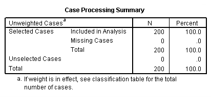
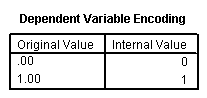
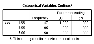
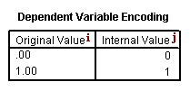
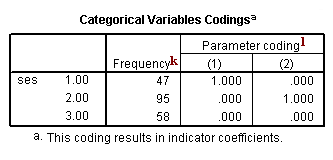
This part of the output tells you about the cases that were included and excluded from the analysis, the coding of the dependent variable, and coding of any categorical variables listed on the categorical subcommand. (Note: You will not get the third table (“Categorical Variable Codings”) if you do not specify the categorical subcommand.)
Logistic Regression
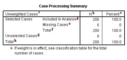
b. N – This is the number of cases in each category (e.g., included in the analysis, missing, total).
c. Percent – This is the percent of cases in each category (e.g., included in the analysis, missing, total).
d. Included in Analysis – This row gives the number and percent of cases that were included in the analysis. Because we have no missing data in our example data set, this also corresponds to the total number of cases.
e. Missing Cases – This row give the number and percent of missing cases. By default, SPSS logistic regression does a listwise deletion of missing data. This means that if there is missing value for any variable in the model, the entire case will be excluded from the analysis.
f. Total – This is the sum of the cases that were included in the analysis and the missing cases. In our example, 200 + 0 = 200.
Unselected Cases – If the select subcommand is used and a logical condition is specified with a categorical variable in the dataset, then the number of unselected cases would be listed here. Using the select subcommand is different from using the filter command. When the select subcommand is used, diagnostic and residual values are computed for all cases in the data. If the filter command is used to select cases to be used in the analysis, residual and diagnostic values are not computed for unselected cases.
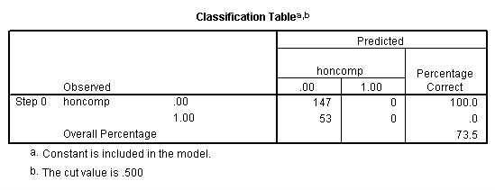
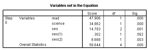
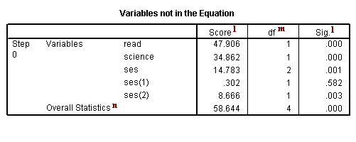
This part of the output describes a “null model”, which is model with no predictors and just the intercept. This is why you will see all of the variables that you put into the model in the table titled “Variables not in the Equation”.
Block 0: Beginning Block
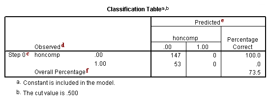

c. Step 0 – SPSS allows you to have different steps in your logistic regression model. The difference between the steps is the predictors that are included. This is similar to blocking variables into groups and then entering them into the equation one group at a time. By default, SPSS logistic regression is run in two steps. The first step, called Step 0, includes no predictors and just the intercept. Often, this model is not interesting to researchers.
d. Observed – This indicates the number of 0’s and 1’s that are observed in the dependent variable.
e. Predicted – In this null model, SPSS has predicted that all cases are 0 on the dependent variable.
f. Overall Percentage – This gives the percent of cases for which the dependent variables was correctly predicted given the model. In this part of the output, this is the null model. 73.5 = 147/200.
g. B – This is the coefficient for the constant (also called the “intercept”) in the null model.
h. S.E. – This is the standard error around the coefficient for the constant.
i. Wald and Sig. – This is the Wald chi-square test that tests the null hypothesis that the constant equals 0. This hypothesis is rejected because the p-value (listed in the column called “Sig.”) is smaller than the critical p-value of .05 (or .01). Hence, we conclude that the constant is not 0. Usually, this finding is not of interest to researchers.
j. df – This is the degrees of freedom for the Wald chi-square test. There is only one degree of freedom because there is only one predictor in the model, namely the constant.
k. Exp(B) – This is the exponentiation of the B coefficient, which is an odds ratio. This value is given by default because odds ratios can be easier to interpret than the coefficient, which is in log-odds units. This is the odds: 53/147 = .361.
l. Score and Sig. – This is a Score test that is used to predict whether or not an independent variable would be significant in the model. Looking at the p-values (located in the column labeled “Sig.”), we can see that each of the predictors would be statistically significant except the first dummy for ses.
m. df – This column lists the degrees of freedom for each variable. Each variable to be entered into the model, e.g., read, science, ses(1) and ses(2), has one degree of freedom, which leads to the total of four shown at the bottom of the column. The variable ses is listed here only to show that if the dummy variables that represent ses were tested simultaneously, the variable ses would be statistically significant.
n. Overall Statistics – This shows the result of including all of the predictors into the model.
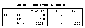
The section contains what is frequently the most interesting part of the output: the overall test of the model (in the “Omnibus Tests of Model Coefficients” table) and the coefficients and odds ratios (in the “Variables in the Equation” table).
Block 1: Method = Enter
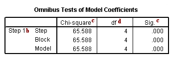
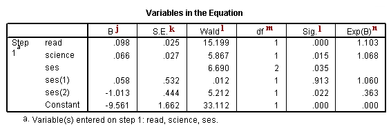
b. Step 1 – This is the first step (or model) with predictors in it. In this case, it is the full model that we specified in the logistic regression command. You can have more steps if you do stepwise or use blocking of variables.
c. Chi-square and Sig. – This is the chi-square statistic and its significance level. In this example, the statistics for the Step, Model and Block are the same because we have not used stepwise logistic regression or blocking. The value given in the Sig. column is the probability of obtaining the chi-square statistic given that the null hypothesis is true. In other words, this is the probability of obtaining this chi-square statistic (65.588) if there is in fact no effect of the independent variables, taken together, on the dependent variable. This is, of course, the p-value, which is compared to a critical value, perhaps .05 or .01 to determine if the overall model is statistically significant. In this case, the model is statistically significant because the p-value is less than .000.
d. df – This is the number of degrees of freedom for the model. There is one degree of freedom for each predictor in the model. In this example, we have four predictors: read, write and two dummies for ses (because there are three levels of ses).
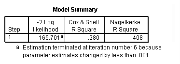
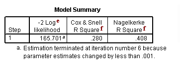
e. -2 Log likelihood – This is the -2 log likelihood for the final model. By itself, this number is not very informative. However, it can be used to compare nested (reduced) models.
f. Cox & Snell R Square and Nagelkerke R Square – These are pseudo R-squares. Logistic regression does not have an equivalent to the R-squared that is found in OLS regression; however, many people have tried to come up with one. There are a wide variety of pseudo-R-square statistics (these are only two of them). Because this statistic does not mean what R-squared means in OLS regression (the proportion of variance explained by the predictors), we suggest interpreting this statistic with great caution.
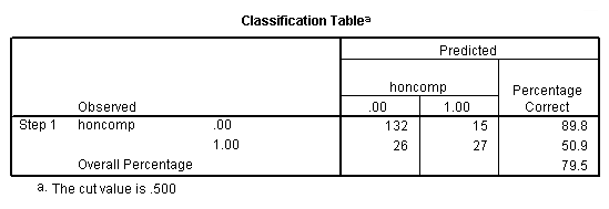
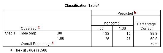
g. Observed – This indicates the number of 0’s and 1’s that are observed in the dependent variable.
h. Predicted – These are the predicted values of the dependent variable based on the full logistic regression model. This table shows how many cases are correctly predicted (132 cases are observed to be 0 and are correctly predicted to be 0; 27 cases are observed to be 1 and are correctly predicted to be 1), and how many cases are not correctly predicted (15 cases are observed to be 0 but are predicted to be 1; 26 cases are observed to be 1 but are predicted to be 0).
i. Overall Percentage – This gives the overall percent of cases that are correctly predicted by the model (in this case, the full model that we specified). As you can see, this percentage has increased from 73.5 for the null model to 79.5 for the full model.
j. B – These are the values for the logistic regression equation for predicting the dependent variable from the independent variable. They are in log-odds units. Similar to OLS regression, the prediction equation is
log(p/1-p) = b0 + b1*x1 + b2*x2 + b3*x3 + b3*x3+b4*x4
where p is the probability of being in honors composition. Expressed in terms of the variables used in this example, the logistic regression equation is
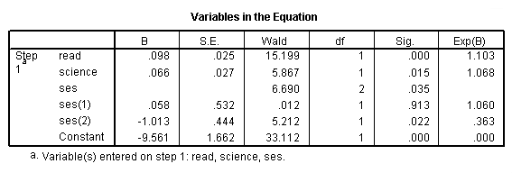
log(p/1-p) = –9.561 + 0.098*read + 0.066*science + 0.058*ses(1) – 1.013*ses(2)
These estimates tell you about the relationship between the independent variables and the dependent variable, where the dependent variable is on the logit scale. These estimates tell the amount of increase (or decrease, if the sign of the coefficient is negative) in the predicted log odds of honcomp = 1 that would be predicted by a 1 unit increase (or decrease) in the predictor, holding all other predictors constant. Note: For the independent variables which are not significant, the coefficients are not significantly different from 0, which should be taken into account when interpreting the coefficients. (See the columns labeled Wald and Sig. regarding testing whether the coefficients are statistically significant). Because these coefficients are in log-odds units, they are often difficult to interpret, so they are often converted into odds ratios. You can do this by hand by exponentiating the coefficient, or by looking at the right-most column in the Variables in the Equation table labeled “Exp(B)”. read – For every one-unit increase in reading score (so, for every additional point on the reading test), we expect a 0.098 increase in the log-odds of honcomp, holding all other independent variables constant. science – For every one-unit increase in science score, we expect a 0.066 increase in the log-odds of honcomp, holding all other independent variables constant. ses – This tells you if the overall variable ses is statistically significant. There is no coefficient listed, because ses is not a variable in the model. Rather, dummy variables which code for ses are in the equation, and those have coefficients. However, as you can see in this example, the coefficient for one of the dummies is statistically significant while the other one is not. The statistic given on this row tells you if the dummies that represent ses, taken together, are statistically significant. Because there are two dummies, this test has two degrees of freedom. This is equivalent to using the test statement in SAS or the test command is Stata. ses(1) – The reference group is level 3 (see the Categorical Variables Codings table above), so this coefficient represents the difference between level 1 of ses and level 3. Note: The number in the parentheses only indicate the number of the dummy variable; it does not tell you anything about which levels of the categorical variable are being compared. For example, if you changed the reference group from level 3 to level 1, the labeling of the dummy variables in the output would not change. ses(2) – The reference group is level 3 (see the Categorical Variables Codings table above), so this coefficient represents the difference between level 2 of ses and level 3. Note: The number in the parentheses only indicate the number of the dummy variable; it does not tell you anything about which levels of the categorical variable are being compared. For example, if you changed the reference group from level 3 to level 1, the labeling of the dummy variables in the output would not change. constant – This is the expected value of the log-odds of honcomp when all of the predictor variables equal zero. In most cases, this is not interesting. Also, oftentimes zero is not a realistic value for a variable to take.
k. S.E. – These are the standard errors associated with the coefficients. The standard error is used for testing whether the parameter is significantly different from 0; by dividing the parameter estimate by the standard error you obtain a t-value. The standard errors can also be used to form a confidence interval for the parameter.
l. Wald and Sig. – These columns provide the Wald chi-square value and 2-tailed p-value used in testing the null hypothesis that the coefficient (parameter) is 0. If you use a 2-tailed test, then you would compare each p-value to your preselected value of alpha. Coefficients having p-values less than alpha are statistically significant. For example, if you chose alpha to be 0.05, coefficients having a p-value of 0.05 or less would be statistically significant (i.e., you can reject the null hypothesis and say that the coefficient is significantly different from 0). If you use a 1-tailed test (i.e., you predict that the parameter will go in a particular direction), then you can divide the p-value by 2 before comparing it to your preselected alpha level. For the variable read, the p-value is .000, so the null hypothesis that the coefficient equals 0 would be rejected. For the variable science, the p-value is .015, so the null hypothesis that the coefficient equals 0 would be rejected. For the variable ses, the p-value is .035, so the null hypothesis that the coefficient equals 0 would be rejected. Because the test of the overall variable is statistically significant, you can look at the one degree of freedom tests for the dummies ses(1) and ses(2). The dummy ses(1) is not statistically significantly different from the dummy ses(3) (which is the omitted, or reference, category), but the dummy ses(2) is statistically significantly different from the dummy ses(3) with a p-value of .022.
m. df – This column lists the degrees of freedom for each of the tests of the coefficients.
n. Exp(B) – These are the odds ratios for the predictors. They are the exponentiation of the coefficients. There is no odds ratio for the variable ses because ses (as a variable with 2 degrees of freedom) was not entered into the logistic regression equation.
Odds Ratios
In this next example, we will illustrate the interpretation of odds ratios. In this example, we will simplify our model so that we have only one predictor, the binary variable female. Before we run the logistic regression, we will use the crosstabs command to obtain a crosstab of the two variables.
crosstabs female by honcomp.
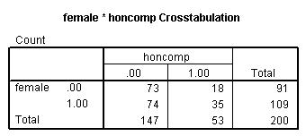
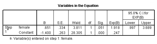
If we divide the number of males who are in honors composition, 18, by the number of males who are not in honors composition, 73, we get the odds of being in honors composition for males, 18/73 = .246. If we do the same thing for females, we get 35/74 = .472. To get the odds ratio, which is the ratio of the two odds that we have just calculated, we get .472/.246 = 1.918. As we can see in the output below, this is exactly the odds ratio we obtain from the logistic regression. The thing to remember here is that you want the group coded as 1 over the group coded as 0, so honcomp=1/honcomp=0 for both males and females, and then the odds for females/odds for males, because the females are coded as 1.
You can get the odds ratio from the crosstabs command by using the /statistics risk subcommand, as shown below.
crosstabs female by honcomp
 /statistics risk.
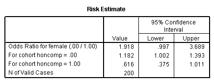
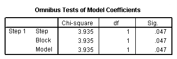
As you can see in the output below, we get the same odds ratio when we run the logistic regression. (NOTE: Although it is equivalent to the odds ratio estimated from the logistic regression, the odds ratio in the “Risk Estimate” table is calculated as the ratio of the odds of honcomp=0 for males over the odds of honcomp=0 for females, which explains the confusing row heading “Odds Ratio for female (.00/1.00)”). If we calculated a 95% confidence interval, we would not want this to include the value of 1. When we were considering the coefficients, we did not want the confidence interval to include 0. If we exponentiate 0, we get 1 (exp(0) = 1). Hence, this is two ways of saying the same thing. As you can see, the 95% confidence interval includes 1; hence, the odds ratio is not statistically significant. Because the lower bound of the 95% confidence interval is so close to 1, the p-value is very close to .05. We can use the /print = ic(95) subcommand to get the 95% confidence intervals included in our output.
There are a few other things to note about the output below. The first is that although we have only one predictor variable, the test for the odds ratio does not match with the overall test of the model. This is because the test of the coefficient is a Wald chi-square test, while the test of the overall model is a likelihood ratio chi-square test. While these two types of chi-square tests are asymptotically equivalent, in small samples they can differ, as they do here. Also, we have the unfortunate situation in which the results of the two tests give different conclusions. This does not happen very often. In a situation like this, it is difficult to know what to conclude. One might consider the power, or one might decide if an odds ratio of this magnitude is important from a clinical or practical standpoint.
logistic regression honcomp with female
 /print = ci(95).
For more information on interpreting odds ratios, please see How do I interpret odds ratios in logistic regression? . Although this FAQ uses Stata for purposes of illustration, the concepts and explanations are useful.
This page shows an example of logistic regression analysis with footnotes explaining the output. These data were collected on 200 high school students and include scores on various tests, including science, math, reading, and social studies (socst). The variable female is a dichotomous variable coded 1 if the student was female and 0 if male.
Because we do not have a suitable dichotomous variable to use as our dependent variable, we will create one (which we will call honcomp, for honors composition) based on the continuous variable write. We do not advocate making dichotomous variables out of continuous variables; rather, we do this here only for purposes of this illustration.
use https://stats.idre.ucla.edu/stat/data/hsb2, clear

generate honcomp = (write >=60)
logit honcomp female read science
Iteration 0:   log likelihood = -115.64441
Iteration 1:   log likelihood = -84.558481
Iteration 2:   log likelihood = -80.491449
Iteration 3:   log likelihood = -80.123052
Iteration 4:   log likelihood = -80.118181
Iteration 5:   log likelihood =  -80.11818

Logit estimates                                   Number of obs   =        200
                                                  LR chi2(3)      =      71.05
                                                  Prob > chi2     =     0.0000
Log likelihood =  -80.11818                       Pseudo R2       =     0.3072

------------------------------------------------------------------------------
     honcomp |      Coef.   Std. Err.      z    P>|z|     [95% Conf. Interval]
-------------+----------------------------------------------------------------
      female |   1.482498   .4473993     3.31   0.001     .6056111    2.359384
        read |   .1035361   .0257662     4.02   0.000     .0530354    .1540369
     science |   .0947902   .0304537     3.11   0.002      .035102    .1544784
       _cons |   -12.7772    1.97586    -6.47   0.000    -16.64982   -8.904589
------------------------------------------------------------------------------
Iteration Log
Iteration 0:   log likelihood = -115.64441
Iteration 1:   log likelihood = -84.558481
Iteration 2:   log likelihood = -80.491449
Iteration 3:   log likelihood = -80.123052
Iteration 4:   log likelihood = -80.118181
Iteration 5:a  log likelihood = -80.11818
a. This is a listing of the log likelihoods at each iteration. (Remember that logistic regression uses maximum likelihood, which is an iterative procedure.) The first iteration (called iteration 0) is the log likelihood of the “null” or “empty” model; that is, a model with no predictors. At the next iteration, the predictor(s) are included in the model. At each iteration, the log likelihood increases because the goal is to maximize the log likelihood. When the difference between successive iterations is very small, the model is said to have “converged”, the iterating is stopped and the results are displayed. For more information on this process, see Regression Models for Categorical and Limited Dependent Variables, Third Edition by J. Scott Long and Jeremy Freese.
Model Summary
Logit estimates                                   Number of obsc   =        200
                                                  LR chi2(3)d      =      71.05
                                                  Prob > chi2e     =     0.0000
Log likelihood =  -80.11818b                      Pseudo R2f       =     0.3072
b. Log likelihood – This is the log likelihood of the final model. The value -80.11818 has no meaning in and of itself; rather, this number can be used to help compare nested models.
c. Number of obs – This is the number of observations that were used in the analysis. This number may be smaller than the total number of observations in your data set if you have missing values for any of the variables used in the logistic regression. Stata uses a listwise deletion by default, which means that if there is a missing value for any variable in the logistic regression, the entire case will be excluded from the analysis.
d. LR chi2(3) – This is the likelihood ratio (LR) chi-square test. The likelihood chi-square test statistic can be calculated by hand as 2*(115.64441 – 80.11818) = 71.05. This is minus two (i.e., -2) times the difference between the starting and ending log likelihood. The number in the parenthesis indicates the number of degrees of freedom. In this model, there are three predictors, so there are three degrees of freedom.
e. Prob > chi2 – This is the probability of obtaining the chi-square statistic given that the null hypothesis is true. In other words, this is the probability of obtaining this chi-square statistic (71.05) if there is in fact no effect of the independent variables, taken together, on the dependent variable. This is, of course, the p-value, which is compared to a critical value, perhaps .05 or .01 to determine if the overall model is statistically significant. In this case, the model is statistically significant because the p-value is less than .000.
f. Pseudo R2 – This is the pseudo R-squared. Logistic regression does not have an equivalent to the R-squared that is found in OLS regression; however, many people have tried to come up with one. There are a wide variety of pseudo-R-square statistics. Because this statistic does not mean what R-square means in OLS regression (the proportion of variance explained by the predictors), we suggest interpreting this statistic with great caution.
Parameter Estimates
------------------------------------------------------------------------------
     honcompg|     Coef.h  Std. Err.i     zj   P>|z|j    [95% Conf. Interval]k
-------------+----------------------------------------------------------------
      female |   1.482498   .4473993     3.31   0.001     .6056111    2.359384
        read |   .1035361   .0257662     4.02   0.000     .0530354    .1540369
     science |   .0947902   .0304537     3.11   0.002      .035102    .1544784
       _cons |   -12.7772    1.97586    -6.47   0.000    -16.64982   -8.904589
------------------------------------------------------------------------------
g. honcomp – This is the dependent variable in our logistic regression. The variables listed below it are the independent variables.
h. Coef. – These are the values for the logistic regression equation for predicting the dependent variable from the independent variable. They are in log-odds units. Similar to OLS regression, the prediction equation is
log(p/1-p) = b0 + b1*female + b2*read + b3*science
where p is the probability of being in honors composition. Expressed in terms of the variables used in this example, the logistic regression equation is
log(p/1-p) = -12.7772 + 1.482498*female + .1035361*read + 0947902*science
These estimates tell you about the relationship between the independent variables and the dependent variable, where the dependent variable is on the logit scale. These estimates tell the amount of increase in the predicted log odds of honcomp = 1 that would be predicted by a 1 unit increase in the predictor, holding all other predictors constant. Note: For the independent variables which are not significant, the coefficients are not significantly different from 0, which should be taken into account when interpreting the coefficients. (See the columns with the z-values and p-values regarding testing whether the coefficients are statistically significant). Because these coefficients are in log-odds units, they are often difficult to interpret, so they are often converted into odds ratios. You can do this by hand by exponentiating the coefficient, or by using the or option with logit command, or by using the logistic command.
female – The coefficient (or parameter estimate) for the variable female is 1.482498. This means that for a one-unit increase in female (in other words, going from male to female), we expect a 1.482498 increase in the log-odds of the dependent variable honcomp, holding all other independent variables constant.
read – For every one-unit increase in reading score (so, for every additional point on the reading test), we expect a .1035361 increase in the log-odds of honcomp, holding all other independent variables constant.
science – For every one-unit increase in science score, we expect a .0947902 increase in the log-odds of honcomp, holding all other independent variables constant.
constant – This is the expected value of the log-odds of honcomp when all of the predictor variables equal zero. In most cases, this is not interesting. Also, oftentimes zero is not a realistic value for a variable to take.
i. Std. Err. – These are the standard errors associated with the coefficients. The standard error is used for testing whether the parameter is significantly different from 0; by dividing the parameter estimate by the standard error you obtain a z-value (see the column with z-values and p-values). The standard errors can also be used to form a confidence interval for the parameter, as shown in the last two columns of this table.
j. z and P>|z| – These columns provide the z-value and 2-tailed p-value used in testing the null hypothesis that the coefficient (parameter) is 0. If you use a 2-tailed test, then you would compare each p-value to your preselected value of alpha. Coefficients having p-values less than alpha are statistically significant. For example, if you chose alpha to be 0.05, coefficients having a p-value of 0.05 or less would be statistically significant (i.e., you can reject the null hypothesis and say that the coefficient is significantly different from 0). If you use a 1-tailed test (i.e., you predict that the parameter will go in a particular direction), then you can divide the p-value by 2 before comparing it to your preselected alpha level. With a 2-tailed test and alpha of 0.05, you may reject the null hypothesis that the coefficient for female is equal to 0. The coefficient of 1.482498 is significantly greater than 0. The coefficient for read is .1035361 significantly different from 0 using alpha of 0.05 because its p-value is 0.000, which is smaller than 0.05. The coefficient for science is .0947902 significantly different from 0 using alpha of 0.05 because its p-value is 0.000, which is smaller than 0.05.
k. [95% Conf. Interval] – This shows a 95% confidence interval for the coefficient. This is very useful as it helps you understand how high and how low the actual population value of the parameter might be. The confidence intervals are related to the p-values such that the coefficient will not be statistically significant if the confidence interval includes 0.
Odds Ratios
In this next example, we will illustrate the interpretation of odds ratios. We will use the logistic command so that we see the odds ratios instead of the coefficients. In this example, we will simplify our model so that we have only one predictor, the binary variable female. Before we run the logistic regression, we will use the tab command to obtain a crosstab of the two variables.
tab female honcomp
           |        honcomp
    female |         0          1 |     Total
-----------+----------------------+----------
      male |        73         18 |        91
    female |        74         35 |       109
-----------+----------------------+----------
     Total |       147         53 |       200
If we divide the number of males who are in honors composition, 18, by the number of males who are not in honors composition, 73, we get the odds of being in honors composition for males, 18/73 = .24657534. If we do the same thing for females, we get 35/74 = .47297297. To get the odds ratio, which is the ratio of the two odds that we have just calculated, we get .47297297/.24657534 = 1.9181682. As we can see in the output below, this is exactly the odds ratio we obtain from the logistic command. The thing to remember here is that you want the group coded as 1 over the group coded as 0, so honcomp=1/honcomp=0 for both males and females, and then the odds for females/odds for males, because the females are coded as 1.
With regard to the 95% confidence interval, we do not want this to include the value of 1. When we were considering the coefficients, we did not want the confidence interval to include 0. If we exponentiate 0, we get 1 (exp(0) = 1). Hence, this is two ways of saying the same thing. As you can see, the 95% confidence interval includes 1; hence, the odds ratio is not statistically significant. Because the lower bound of the 95% confidence interval is so close to 1, the p-value is very close to .05.
There are a few other things to note about the output below. The first is that although we have only one predictor variable, the test for the odds ratio does not match with the overall test of the model. This is because the z statistic is actually the result of a Wald chi-square test, while the test of the overall model is a likelihood ratio chi-square. While these two types of chi-square tests are asymptotically equivalent, in small samples they can differ, as they do here. Also, we have the unfortunate situation in which the results of the two tests give different conclusions. This does not happen very often. In a situation like this, it is difficult to know what to conclude. One might consider the power, or one might decide if an odds ratio of this magnitude is important from a clinical or practical standpoint.
logistic honcomp female
Logistic regression                               Number of obs   =        200
                                                  LR chi2(1)      =       3.94
                                                  Prob > chi2     =     0.0473
Log likelihood =  -113.6769                       Pseudo R2       =     0.0170

------------------------------------------------------------------------------
     honcomp | Odds Ratio   Std. Err.      z    P>|z|     [95% Conf. Interval]
-------------+----------------------------------------------------------------
      female |   1.918168   .6400451     1.95   0.051     .9973827    3.689024
------------------------------------------------------------------------------
For more information on interpreting odds ratios, please see How do I interpret odds ratios in logistic regression? .